Applications of the Soave-Redlich-Kwong Equation of State
Housam Binous and Ahmed Bellagi
Applications of the Soave-Redlich-Kwong Equation of State
Housam Binous and Ahmed Bellagi
Housam Binous and Ahmed Bellagi
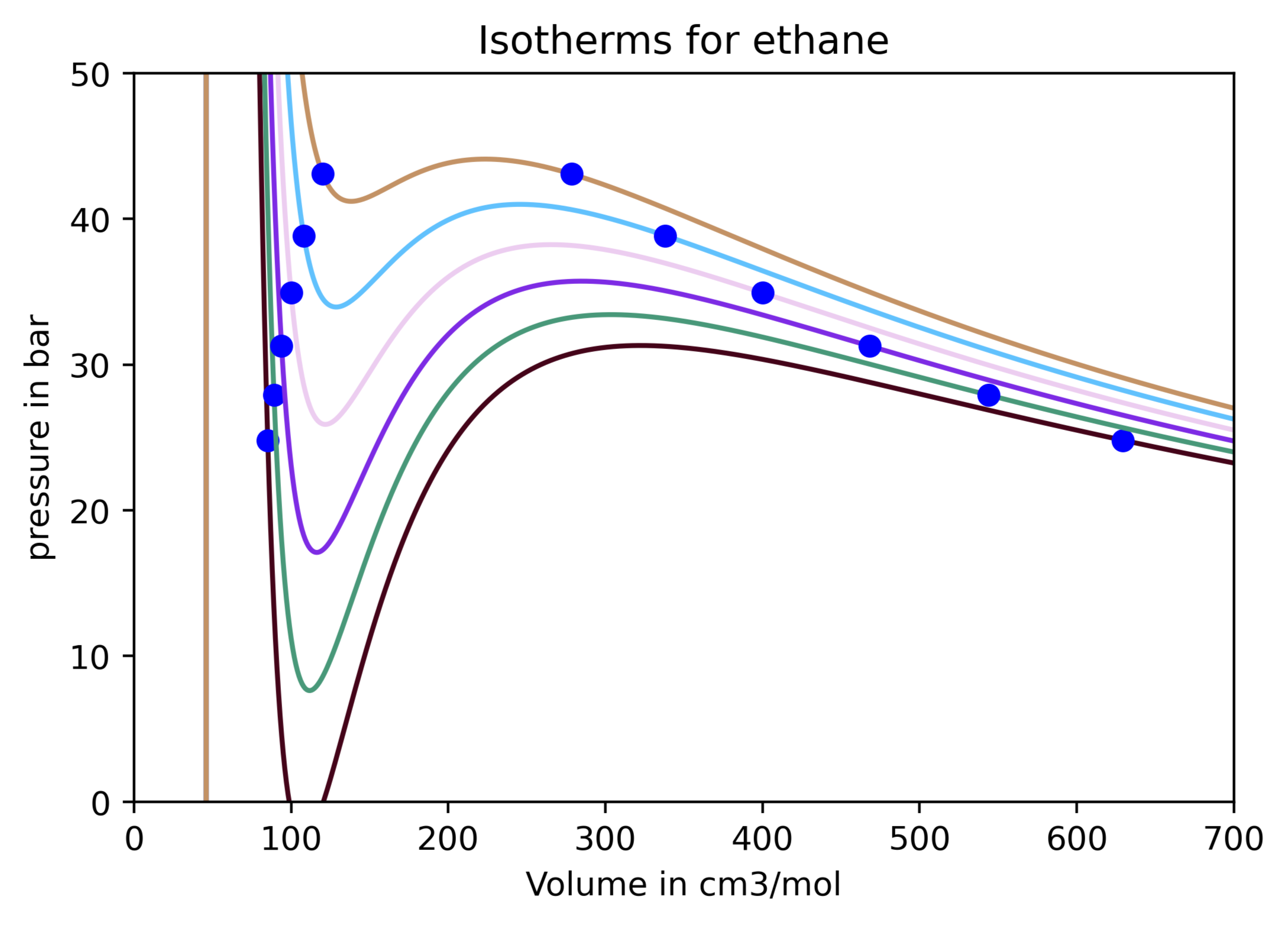
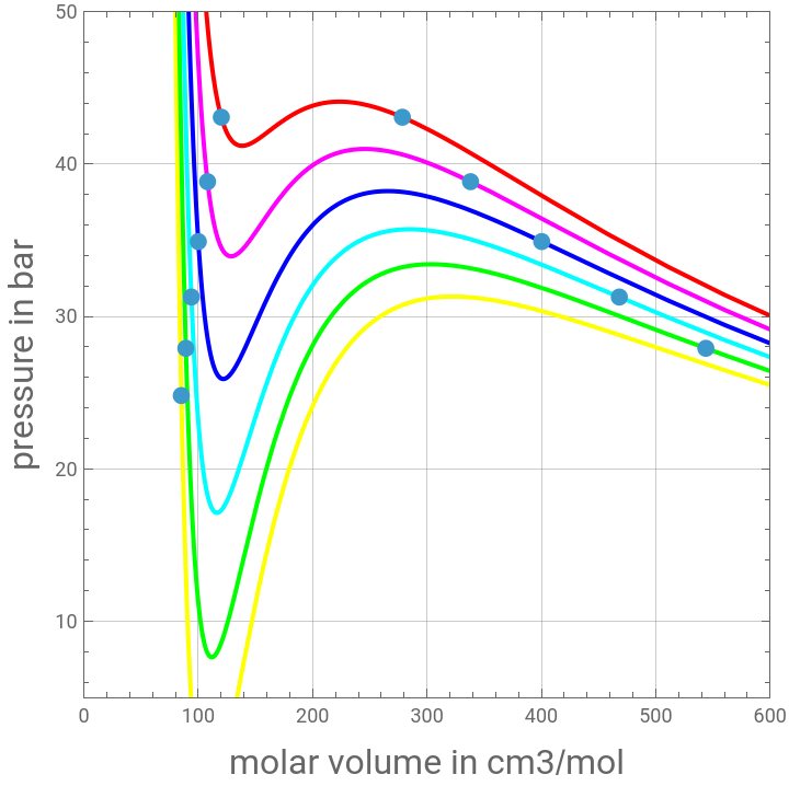
The present calculations were published in Ref. 1. Here, we show how one can use the Soave-Redlich-Kwong Equation of State to compute vapor and liquid molar volumes and vapor pressure at various temperatures as well as the vapor liquid equilibrium curve for Ethane. The vapor pressure data obtained using this cubic equation of state are compared with success to the results derived from the modified Antoine’s equation (based on Aspen-Hysys).
Reference:
[1] Zakia Nasri, Housam Binous, Applications of the Soave–Redlich–Kwong Equation of State Using Mathematica®, Journal of Chemical Engineering of Japan, 2007, Volume 40, Issue 6, Pages 534-538
Acknowledgement :
This problem was presented in the Master's report of R. Privat under the direction of J-P Corriou at ENSIC, Nancy, France.
Reduced Temperature
In[]:=
Tre=(θ+273.15)/Tc;
Ethane's Critical Pressure, Critical Temperature and Acentric Factor. R is the Universal Gas Constant
In[]:=
Tc=273.15+32.28;Pc=48.84;ω=0.09860;R=83.14;
Soave-Redlich-Kwong Equation of State
In[]:=
P[T_,v_]:=RT/(v-b)-a/(v(v+b))
In[]:=
b=0.08664RTc/Pc
Out[]=
45.0469
In[]:=
m=0.480+1.574ω-0.176ω^2
Out[]=
0.633485
In[]:=
a=0.42748(RTc)^2/Pc1+m1-
Tre
^2Out[]=
5.64396×
6
10
2
1+0.6334851-0.0572195
273.15+θ
In[]:=
tbl=Table[P[θ+273.15,v],{θ,1,30,5}];
Plotting Isotherms
In[]:=
plt[θ_]:=Plot[tbl[[θ]],{v,0,2500},PlotRange{{0,2500},{0,100}},PlotStyleHue[θ/6],Frame->True,GridLines->Automatic,AspectRatio->1]
In[]:=
plot1=Show[Table[plt[θ],{θ,1,6}],FrameLabel->{Style["molar volume in cm3/mol",16],Style["pressure in bar",16]}]
Out[]=
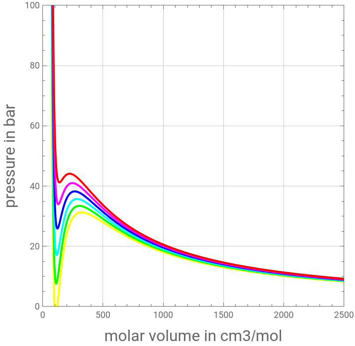
Finding vapor pressure and liquid and gas molar volumes at different temperatures. Dots in the figure show vapor liquid equilibrium curve for ethane.PythonMathematica
In[]:=
sol[θ_?NumericQ]:=Quiet@FindRoot[{NIntegrate[-P[273.15+θ,v]+P[273.15+θ,x],{v,x,z}]NIntegrate[P[273.15+θ,v]-P[273.15+θ,y],{v,z,y}],P[273.15+θ,x]P[273.15+θ,z],P[273.15+θ,z]P[273.15+θ,y]},{x,50},{z,120},{y,400},MaxIterations->100]
In[]:=
tbl1=Quiet@Table[{x,P[θ+273.15,x]}/.sol[θ],{θ,1,30,5}]
Out[]=
{{85.1397,24.8124},{89.1129,27.9134},{93.9325,31.2787},{99.9972,34.9205},{108.085,38.8506},{120.123,43.0813}}
In[]:=
tbl2=Quiet@Table[{y,P[θ+273.15,y]}/.sol[θ],{θ,1,30,5}]
Out[]=
{{629.251,24.8124},{543.734,27.9134},{468.08,31.2787},{400.224,34.9205},{338.019,38.8506},{278.409,43.0813}}
In[]:=
TBL=Join[tbl1,Sort[tbl2]]
Out[]=
{{85.1397,24.8124},{89.1129,27.9134},{93.9325,31.2787},{99.9972,34.9205},{108.085,38.8506},{120.123,43.0813},{278.409,43.0813},{338.019,38.8506},{400.224,34.9205},{468.08,31.2787},{543.734,27.9134},{629.251,24.8124}}
In[]:=
plot2=ListPlot[TBL,PlotStylePointSize[0.025],Frame->True,GridLines->Automatic,AspectRatio->1];
In[]:=
Show[plot1,plot2,PlotRange{{0,600},{5,50}}]
Out[]=
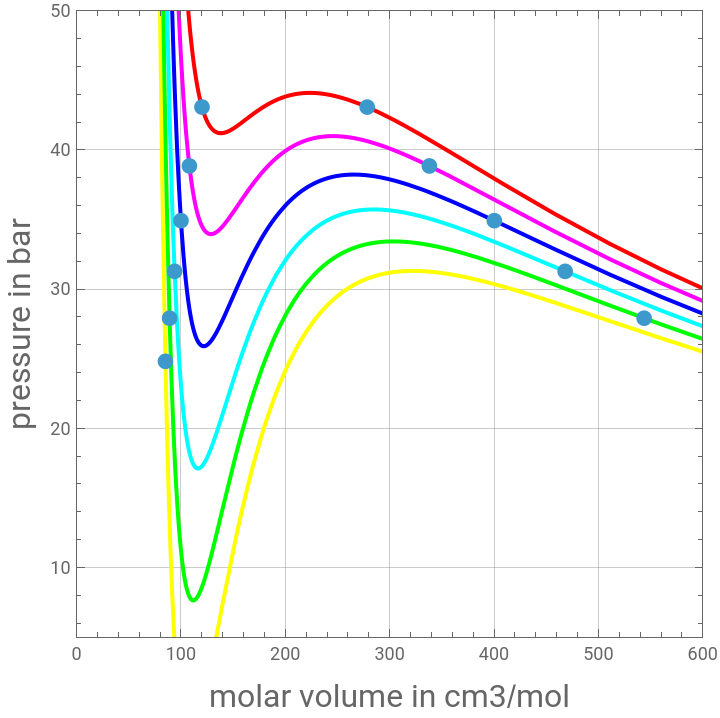
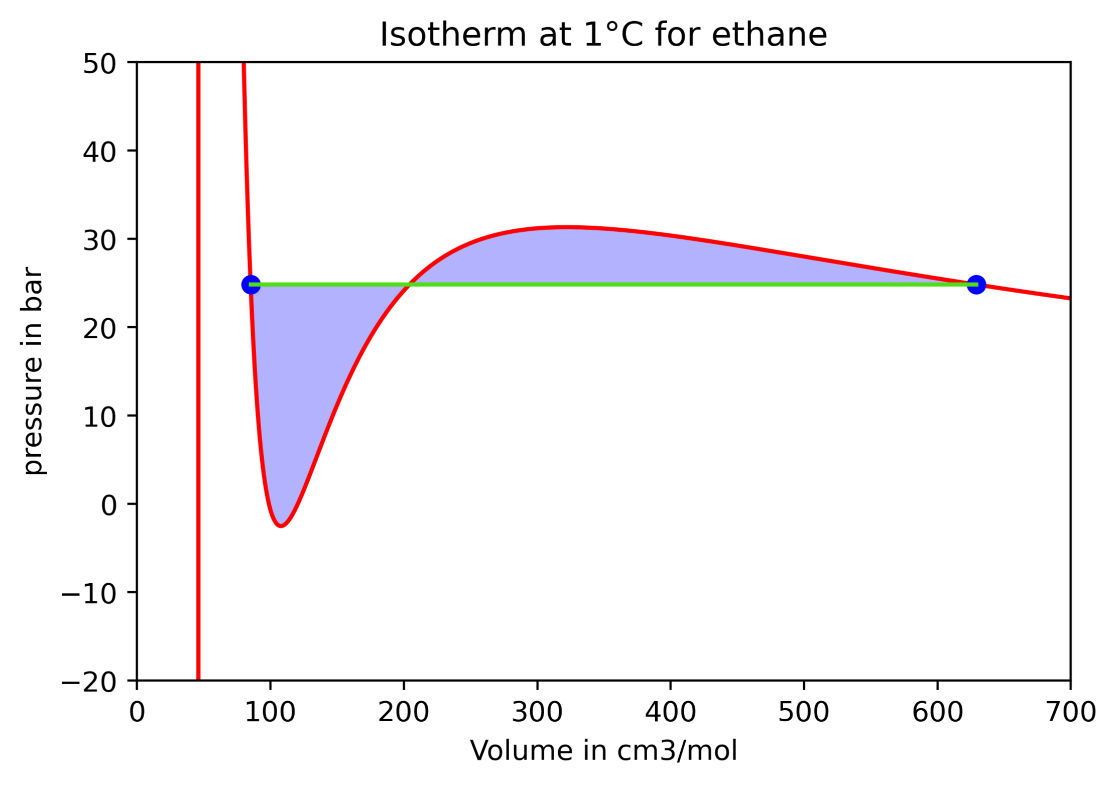
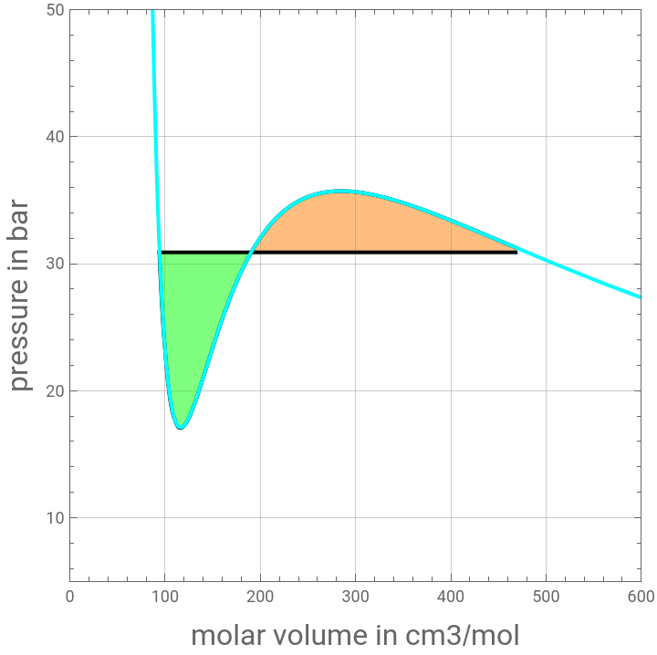
The equilibrium data is obtained by solving a system of equation so that the two areas are equal.Python (python coding is provided at the end of the notebook)Mathematica
Checking Maxwell' s Equal Area Rule
Modified Antoine's equation obtained from Aspen-HYSYS
Antoine's equation obtained from Equilibrium-Stage Separation Operations in Chemical Engineering by Henley and Seader, Wiley, 1981.
Python coding