Riordan Arrays for the enumeration of combinatorial structures
Applications to statistics
by Jan Greve (Mentor: Christopher Wolfram)
WU Vienna University of Economics and Business
Applications to statistics
by Jan Greve (Mentor: Christopher Wolfram)
WU Vienna University of Economics and Business
The aim of this project is to implement various operations on the Riordan array with the specific goal to address statistical problems. A Riordan array is a special type of matrix utilized primarily in combinatorics to represent various combinatorial identities in a principled manner. It is particularly suited to tackle the enumeration problem of combinatorial structures such as (set or integer) partitions, lattice walks, trees, graphs, etc., that are defined recursively based on a set of rules. As an example of a recursively defined combinatorial object with statistical importance, consider the process of splitting a tree. Such a process represented as a cladogram is usually defined in a recursive manner, and its stochastic variant called Markov branching forms an important theoretical foundation for population genetics. The advantage of using Mathematica in this project has to do with the fact that various computations involving Riordan arrays result in operations such as the transformation of characteristic generating functions of the Riordan array, extraction of relevant coefficients from the resulting generating function, etc., which are best handled symbolically. What follows in this notebook is a brief sketch of relevant features of the Riordan array all coupled with a Mathematica code and the corresponding output. In addition, one illustrative example in statistics will be shown at the end followed by a remark about limitations in the current implementation and future work.
Definition and property of the Riordan array
Definition and property of the Riordan array
Characterization of the Riordan array by a pair of formal power series
Characterization of the Riordan array by a pair of formal power series
Consider a pair of formal power series:
g(t)=+t++⋯
g
0
g
1
g
2
2
t
f
1
f
2
2
t
(
1
)with !=0. The Riordan Array is fully described by such in the following manner. Let -th element of the Riordan array defined as , then we have:
g
0
f
1
(g(t),f(t))
(n,k)
ℛ
d
n,k
d
n,k
n
t
k
f(t)
(
2
)for all (note that the indexing of the Riordan array starts at 0, not 1) where refers to the operator of taking the coefficient of the term .Immediately, we notice that =0 for making the Riordan array lower-triangular. In addition, as both and contain infinitely many terms, the Riordan array is a matrix.From here on, the dimensional lower-triangular Riordan array characterized by the pair of formal power series will be referred to as .
n,k∈
0
[]
n
t
n
t
d
n,k
k=n+1,n+2,…
ℛ
g(t)
f(t)
ℛ
∞∞
∞∞
(g(t),f(t))
ℛ(g(t),f(t))
Example 1:
Identity matrix, because
Identity matrix
ℛ(g(t)=1,f(t)=t)
d
n,k
n
t
k
t
δ
n,k
The Mathematica implementation of this object called the object is defined with a pair of pure functions corresponding to and .
RiordanArray
g(t)=1
f(t)=t
In[]:=
RiordanArray[(1)&,(#)&]
Out[]=
RiordanArray

where the heat map used as an icon of the object represents the values of the first few dimensions.
For this object, the function is extended to specifically evaluate dimensions (in rows and columns) in the specified range and add padding to the appropriate positions with values that are outside the specified range.
RiordanArray
For this object, the
MatrixForm
In[]:=
MatrixForm[RiordanArray[(1)&,(#)&],{0;;5,0;;5}]
Out[]//MatrixForm=
1 | 0 | 0 | 0 | 0 | 0 | ⋯ |
0 | 1 | 0 | 0 | 0 | 0 | ⋯ |
0 | 0 | 1 | 0 | 0 | 0 | ⋯ |
0 | 0 | 0 | 1 | 0 | 0 | ⋯ |
0 | 0 | 0 | 0 | 1 | 0 | ⋯ |
0 | 0 | 0 | 0 | 0 | 1 | ⋯ |
⋮ | ⋮ | ⋮ | ⋮ | ⋮ | ⋮ | ⋱ |
Of course, the object can be parted in the usual way which returns a list of lists, a format more suitable for further manipulations if needed.
RiordanArray
In[]:=
RiordanArray[(1)&,(#)&][0;;5,0;;5]
Out[]=
{{1,0,0,0,0,0},{0,1,0,0,0,0},{0,0,1,0,0,0},{0,0,0,1,0,0},{0,0,0,0,1,0},{0,0,0,0,0,1}}
Further aspects of the Riordan array involving the column generating function
Further aspects of the Riordan array involving the column generating function
Another way to look at the Riordan array is to think of it as a sequence of column generating functions
g(t),g(t)f(t),g(t),…
2
f(t)
(
3
)following the geometric progression. To highlight this aspect of the Riordan array, the accessor function called is implemented to obtain the -th column generating function as a pure function or as a series depending on the optional argument.
ColumnGeneratingFunction
k
Example 2 :Pascal’s triangle =[]*=[](1-t) =[] = =[]1+t++⋯++⋯ =
ℛg(t)=,f(t)=
1
1-t
t
1-t
d
n,k
n
t
1
1-t
k
t
1-t
n
t
-(k+1)
k
t
n-k
t
-(k+1)
(1-t)
[]
n-k
t
k+1
(1+t++⋯)
2
t
n-k
t
(k+1)!
1!k!
(k+2)!
2!k!
2
t
n!
k!(n-k)!
n-k
t
n!
k!(n-k)!
In[]:=
ColumnGeneratingFunction[RiordanArray[(1/(1-#))&,(#/(1-#))&],5][t]
Out[]=
5
t
6
(1-t)
In[]:=
ColumnGeneratingFunction[RiordanArray[(1/(1-#))&,(#/(1-#))&],5,{t,10}]
Out[]=
5
t
6
t
7
t
8
t
9
t
10
t
11
O[t]
From the dimensional subset of the Pascal’s triangle shown below, we can verify the validity of the generating function above (coefficients represent the numbers in the matrix at the corresponding row).
1010
In[]:=
MatrixForm[RiordanArray[(1/(1-#))&,(#/(1-#))&],{0;;10,0;;10}]
Out[]//MatrixForm=
1 | 0 | 0 | 0 | 0 | 0 | 0 | 0 | 0 | 0 | 0 | ⋯ |
1 | 1 | 0 | 0 | 0 | 0 | 0 | 0 | 0 | 0 | 0 | ⋯ |
1 | 2 | 1 | 0 | 0 | 0 | 0 | 0 | 0 | 0 | 0 | ⋯ |
1 | 3 | 3 | 1 | 0 | 0 | 0 | 0 | 0 | 0 | 0 | ⋯ |
1 | 4 | 6 | 4 | 1 | 0 | 0 | 0 | 0 | 0 | 0 | ⋯ |
1 | 5 | 10 | 10 | 5 | 1 | 0 | 0 | 0 | 0 | 0 | ⋯ |
1 | 6 | 15 | 20 | 15 | 6 | 1 | 0 | 0 | 0 | 0 | ⋯ |
1 | 7 | 21 | 35 | 35 | 21 | 7 | 1 | 0 | 0 | 0 | ⋯ |
1 | 8 | 28 | 56 | 70 | 56 | 28 | 8 | 1 | 0 | 0 | ⋯ |
1 | 9 | 36 | 84 | 126 | 126 | 84 | 36 | 9 | 1 | 0 | ⋯ |
1 | 10 | 45 | 120 | 210 | 252 | 210 | 120 | 45 | 10 | 1 | ⋯ |
⋮ | ⋮ | ⋮ | ⋮ | ⋮ | ⋮ | ⋮ | ⋮ | ⋮ | ⋮ | ⋮ | ⋱ |
Riordan group
Riordan group
The set of all Riordan arrays is closed under matrix multiplication (i.e., dot product) and the operation is associative.
The matrix multiplication of two Riordan arrays, is defined as:
The matrix multiplication of two Riordan arrays
ℛ((t),(t))
g
1
f
1
ℛ((t),(t))
g
2
f
2
ℛ((t),(t))*ℛ((t),(t))=ℛ((t)((t)),((t))).
g
1
f
1
g
2
f
2
g
1
g
2
f
1
f
2
f
1
(
4
)The identity array is (as already shown in Example 1), and the inverse exists uniquely for each which is also a Riordan array defined as follows:
ℛ(1,t)
ℛ(g(t),f(t))
-1
ℛ(g(t),f(t))
1
g((t))
f
f
f((t))=(f(t))=t
f
f
(
5
)that is, (t) is the compositional inverse of . One can easily check by plugging in in Equation to one of the terms in Equation to see that the resulting multiplication returns an identity Riordan array .Hence, the set of all Riordan arrays form a group under matrix multiplication.
f
f(t)
-1
ℛ(g(t),f(t))
(5)
(4)
ℛ(1,t)
Multiplication (dot product) between two objects is implemented in Mathematica as follows:
RiordanArray
In[]:=
RiordanArray[(1)&,(#)&].RiordanArray[(1/(1-#))&,(#/(1-#))&]
Out[]=
RiordanArray

we see that the product of the identity matrix and the Pascal’s triangle is the Pascal’s triangle itself.Inverse of the object can be obtained by simply calling the as follows:
ℛ(1,t)
ℛ,
1
1-t
t
1-t
RiordanArray
Inverse
In[]:=
Inverse[RiordanArray[(1/(1-#))&,(#/(1-#))&]]
Out[]=
RiordanArray
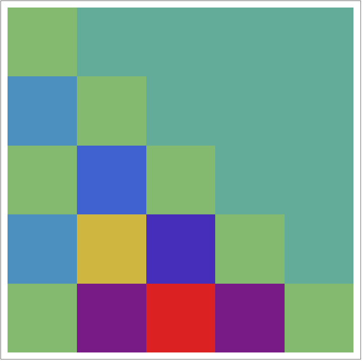
In[]:=
MatrixForm[%,{0;;10,0;;10}]
Out[]//MatrixForm=
1 | 0 | 0 | 0 | 0 | 0 | 0 | 0 | 0 | 0 | 0 | ⋯ |
-1 | 1 | 0 | 0 | 0 | 0 | 0 | 0 | 0 | 0 | 0 | ⋯ |
1 | -2 | 1 | 0 | 0 | 0 | 0 | 0 | 0 | 0 | 0 | ⋯ |
-1 | 3 | -3 | 1 | 0 | 0 | 0 | 0 | 0 | 0 | 0 | ⋯ |
1 | -4 | 6 | -4 | 1 | 0 | 0 | 0 | 0 | 0 | 0 | ⋯ |
-1 | 5 | -10 | 10 | -5 | 1 | 0 | 0 | 0 | 0 | 0 | ⋯ |
1 | -6 | 15 | -20 | 15 | -6 | 1 | 0 | 0 | 0 | 0 | ⋯ |
-1 | 7 | -21 | 35 | -35 | 21 | -7 | 1 | 0 | 0 | 0 | ⋯ |
1 | -8 | 28 | -56 | 70 | -56 | 28 | -8 | 1 | 0 | 0 | ⋯ |
-1 | 9 | -36 | 84 | -126 | 126 | -84 | 36 | -9 | 1 | 0 | ⋯ |
1 | -10 | 45 | -120 | 210 | -252 | 210 | -120 | 45 | -10 | 1 | ⋯ |
⋮ | ⋮ | ⋮ | ⋮ | ⋮ | ⋮ | ⋮ | ⋮ | ⋮ | ⋮ | ⋮ | ⋱ |
We can verify that the resulting inverse of the Pascal’s triangle is correct by the multiplication with its own
In[]:=
Inverse[RiordanArray[(1/(1-#))&,(#/(1-#))&]].RiordanArray[(1/(1-#))&,(#/(1-#))&]
Out[]=
RiordanArray
which results in an identity array once simplifying the .
As a conscious design choice, simplification of and is not automatically done. This is because a more complicated inversion and/or matrix multiplication of Riordan arrays often involving symbolic variables require a user intervention for the simplification to be done right (such as restricting the range of symbolic variables accordingly, etc.).
To carry out a proper simplification of and/or , an accessor function can be utilized.
ℛ(1,t)
f(t)
As a conscious design choice, simplification of
g(t)
f(t)
To carry out a proper simplification of
g(t)
f(t)
GetGeneratingFunctionPairs
Fundamental Theorem of Riordan Arrays (FTRA)
Fundamental Theorem of Riordan Arrays (FTRA)
In terms of generating function, it is often written as
First, consider enumerating the 1001-th row sum in the naive manner:
Alternative characterization of the Riordan array
Alternative characterization of the Riordan array
Riordan arrays can be considered a generalization of the Pascal’s triangle with the property
As we can see, we get the intended results from these functions.
Application: Lattice walk counting and its use in statistics
Application: Lattice walk counting and its use in statistics
Problem description
Problem description
NOTE:This example is from the book [2] but the way to develop this combinatorial problem into something meaningful in statistics is author’s own idea.
where
We can enumerate all such paths by an ordered labeled tree following the rule:
The use of Riordan arrays to tackle this problem
The use of Riordan arrays to tackle this problem
Assuming that this lattice path can be represented by an element in the Riordan array, the branching rule of the tree can be written as follows:
Application to statistics
Application to statistics
To turn this into a probability distribution on all terminating nodes following the above rule, one can simply divide each row by the row sums which enumerates all possible paths following this rule. For this matrix, one can simply do the following:
Some remarks about the use of Riordan arrays to generate random combinatorial structures
Some remarks about the use of Riordan arrays to generate random combinatorial structures
Conclusion
Conclusion
Riordan arrays provide concise and computationally efficient ways of enumerating various combinatorial objects that are defined recursively. As a by-product, it is extremely easy to define random combinatorial structures using the Riordan array although it does not necessarily respect the various constraints these structures need to meet in order to be statistically meaningful. However, this may open up an interesting avenue of future research where these constraints, known for each random combinatorial structure, are to be unified under the general framework of Riordan arrays. In any case, an implementation of various operations carried out on Riordan arrays requires a symbolic implementation and Mathematica is perfectly suited for this task.
Limitations and future work
Limitations and future work
The issue of sampling consistency has been well explored for various models including the random cladograms. How these theoretical results translates to the aforementioned way of utilizing Riordan arrays to define random combinatorial objects is an interesting avenue of future research.
All the functionalities in this community post will eventually be packaged under the name “RiordanArray`” and distributed in the Wolfram paclet repository.
Keywords
Keywords
Random Combinatorial Structures
Riordan Arrays
Statistics
Enumerative Combinatorics
Acknowledgement
Acknowledgement
First and foremost, I thank my mentor Christopher Wolfram for his consistent support throughout the duration of the WSS22 as my mentor. Without his advice, it would have been impossible to implement all these features I envisioned to implement in the Mathematica when I started this project. His extensive knowledge in symbolic computing and constructive comments regarding the various functionalities I implemented has allowed me to create a comprehensive set of functions that deals with the Riordan array -- a promising new development in the combinatorics --. Furthermore, I thank Stephen Wolfram for his understanding of my objective to pursue my own research ideas and many of his thought-provoking guidance during the meetings. Finally, I thank everyone in the WSS22 from organizers, mentors to fellow participants for this wonderful opportunity to learn and work together in a intellectually stimulating and inclusive environment.
References
References
[1] Aldous, D. Probability distributions on cladograms. Random discrete structures, Springer, New York, NY, (1996). 1-18.
[2] Shapiro, L., Sprugnoli, R., Barry, P., Cheon, G. S., He, T. X., Merlini, D., & Wang, W. The Riordan Group and Applications, Springer Monographs in Mathematics, (2022).
Appendix
Appendix