I have had the privilege of knowing Dr. Paul Abbott since 2018 when he mentored me at the Wolfram Summer School. Despite our limited interactions, each engagement has been invaluable, both personally and professionally. Recently, he recommended the paper Schrödinger cat states of a nuclear spin qudit in silicon and suggested its implementation in the Wolfram Quantum Framework, which we have been developing for several years. Here is the result.
One way to construct the discrete Wigner function is to represent the density matrix in the basis of irreducible spherical tensors as follows: where is the spin (the dimension of space is ), (θ,ϕ) are spherical harmonics, and are density matrix element in the basis of irreducible spherical tensor, .
(θ,ϕ)=(θ,ϕ)
2
π
2j
∑
k=0
k
∑
q=-k
q
Y
k
ρ
kq
j
1+2j
q
Y
k
ρ
kq
q
k
Install Wolfram quantum framework
In[]:=
PacletInstall[CloudObject["https://wolfr.am/DevWQCF"],ForceVersionInstall->True]<<Wolfram`QuantumFramework`
Out[]=
PacletObject

Construct matrices and operators corresponding to irreducible spherical tensor, (j):
q
k
In[]:=
ClearAll[TkqMatrix,TkqOperator]TkqMatrix[j_,{k_Integer,q_Integer}]/;0<=k<=2j&&-k<=q<=k:=SparseArray[{mi_,mj_}/;mj==mi-q:>With[{m1=mi-j-1},(-1)^(j-m1)(2k+1)^(1/2)ThreeJSymbol[{j,-m1},{k,q},{j,m1-q}]],{2j+1,2j+1}]TkqOperator[j_,{k_Integer,q_Integer}]/;0<=k<=2j&&-k<=q<=k:=QuantumOperator[TkqMatrix[j,{k,q}],QuantumBasis["JZ"[j]]]
q
1
(-1)
q
1
k
1
q
2
k
2
δ
k
1
k
2
δ
q,
q
2
In[]:=
(*setthespin*)j=5/2;(*checktheaboverelationshipforallvaluesofand*)Table[Tr[(-1)^q1TkqMatrix[j,{k1,-q1}].TkqMatrix[j,{k2,q2}]]==KroneckerDelta[k1,k2]KroneckerDelta[q1,q2],{k1,0,2j},{q1,-k1,k1},{k2,0,2j},{q2,-k2,k2}]//Flatten//Apply[And]
q
i
k
i
Out[]=
True
Set the spin to 7/2, corresponding to an 8-dimensional Hilbert space, as in the paper.
In[]:=
j=7/2;
(θ,ϕ)=(θ,ϕ)
2
π
2j
∑
k=0
k
∑
q=-k
q
Y
k
ρ
kq
In[]:=
ClearAll[phaseSpaceWigner]phaseSpaceWigner[state_]:=QuantumPhaseSpaceTransform[state,QuantumBasis[Flatten[Table[TkqMatrix[j,{k,q}],{k,0,2j},{q,-k,k}],1]]]["StateVector"].Flatten[Table[SphericalHarmonicY[k,q,θ,φ],{k,0,2j},{q,-k,k}],1]//N//Re
2
π
For the sake of plotting and its coloring, find min and max values of Wigner function:
In[]:=
ClearAll[minmax]minmax[w_]:={NMinimize[{w,0<=θ<=π,0<=φ<=2π},{θ,φ}][[1]],NMaximize[{w,0<=θ<=π,0<=φ<=2π},{θ,φ}][[1]]}
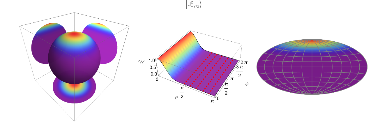
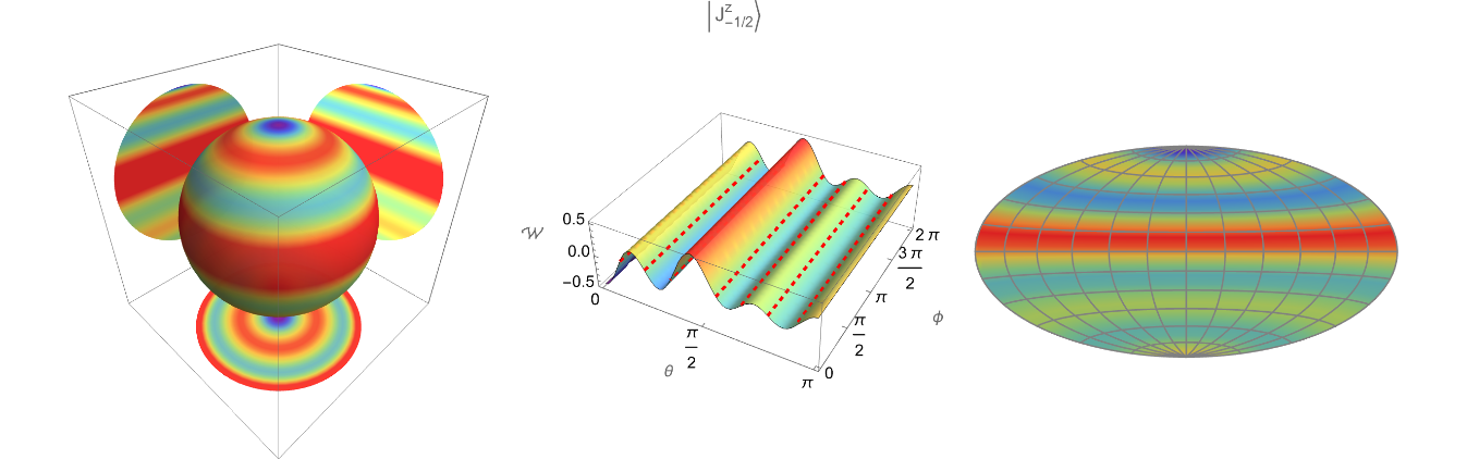
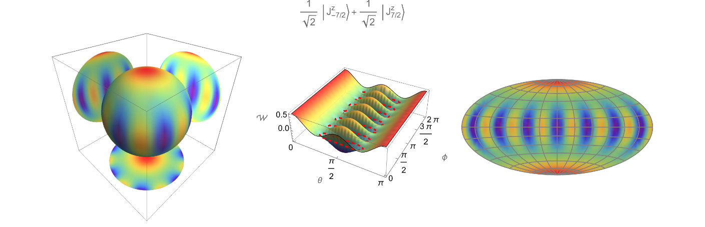
Since θ and ϕ are spherical angles, the plot can happen either on a sphere, or its 2D projection, such as Hammer projection:
In[]:=
ClearAll[convertSphericalToLatLon,hammerPlotGeo]convertSphericalToLatLon[{theta_,phi_}]:={90-theta180/π,phi180/π}Options[hammerPlotGeo]=Options[GeoDensityPlot];SetOptions[hammerPlotGeo,GeoProjection->"Hammer",GeoBackground->None,GeoGridLines->Automatic,GeoGridLinesStyle->Directive[Gray],ColorFunction->"Rainbow",PlotRange->All];hammerPlotGeo[fun_,opts:OptionsPattern[]]:=GeoDensityPlot[GeoPosition[#1]->#2&@@Transpose[Flatten[Outer[{convertSphericalToLatLon[{#1,#2}],fun[#1,#2]}&,Range[0,π,π/25],Range[0,2π,π/25]],1]],Evaluate[FilterRules[{opts,Options[hammerPlotGeo]},Options[GeoDensityPlot]]]]
A function to have 3 different visualization of the Wigner function:
In[]:=
ClearAll[visualize]visualize[wignerFunction_,range_]:={Show[{ParametricPlot3D[{Cos[φ]Sin[θ],Sin[θ]Sin[φ],Cos[θ]},{θ,0,Pi},{φ,-Pi,Pi},Mesh->None,PlotStyle->Opacity[.9],ColorFunction->Function[ColorData["Rainbow"][Rescale[wignerFunction[#4,#5],range]]],ColorFunctionScaling->False,PlotPoints->50],ParametricPlot3D[{-1.5,Sin[θ]Sin[φ],Cos[θ]},{θ,0,Pi},{φ,-Pi,Pi},Mesh->None,PlotStyle->Opacity[.9],ColorFunction->Function[ColorData["Rainbow"][Rescale[wignerFunction[#4,ArcTan[-Cos[#5],Sin[#5]]],range]]],ColorFunctionScaling->False,PlotPoints->50],ParametricPlot3D[{Cos[φ]Sin[θ],1.5,Cos[θ]},{θ,0,Pi},{φ,-Pi,Pi},Mesh->None,PlotStyle->Opacity[.9],ColorFunction->Function[ColorData["Rainbow"][Rescale[wignerFunction[#4,ArcTan[Cos[#5],-Sin[#5]]],range]]],ColorFunctionScaling->False,PlotPoints->50,Lighting->DirectionalLight[White,{{0,0,0},{0,1.5,0}}]],ParametricPlot3D[{Cos[φ]Sin[θ],Sin[θ]Sin[φ],-1.5},{θ,0,Pi},{φ,-Pi,Pi},Mesh->None,PlotStyle->Opacity[.9],ColorFunction->Function[ColorData["Rainbow"][Rescale[wignerFunction[ArcTan[Cos[#4],-Sin[#4]],#5],range]]],ColorFunctionScaling->False,PlotPoints->50]},ViewPoint->{1,-1,1},Boxed->True,PlotRange->All,Ticks->None,ImageSize->300],Plot3D[wignerFunction[θ,φ],{θ,0,Pi},{φ,0,2Pi},Mesh->{{{0,Directive[Dashed,Thick,Red]}}},MeshFunctions->{#3&},ColorFunction->"Rainbow",BoxRatios->{1,1,1/3},PlotStyle->Opacity[.9],PlotRange->All,Ticks->{Range[0,2π,π/2],Range[0,2π,π/2],Automatic},AxesLabel->{"θ","ϕ",""},ImageSize->300],(*Quiet@HammerPlot[wignerFunction,ColorFunction->"Rainbow",PlotPoints->100,ImageSize->300]*)hammerPlotGeo[wignerFunction,OpacityFunctionNone,ImageSize->300]}
Show Wigner function for some states:
In[]:=
state=QuantumState["0","JZ"[j]];w=phaseSpaceWigner[state];range=minmax[w];Show[GraphicsRow[visualize[{θ,φ}|->Evaluate[w],range]],PlotLabel->TraditionalForm[state]]
Out[]=
In[]:=
state=QuantumState["3","JZ"[j]];w=phaseSpaceWigner[state];range=minmax[w];Show[GraphicsRow[visualize[{θ,φ}|->Evaluate[w],range]],PlotLabel->TraditionalForm[state]]
Out[]=
In[]:=
state=;w=phaseSpaceWigner[state];range=minmax[w];Show[GraphicsRow[visualize[{θ,φ}|->Evaluate[w],range]],PlotLabel->TraditionalForm[state]]
QuantumState["0","JZ"[j]]+QuantumState[ToString[2j+1],"JZ"[j]]
2
Out[]=
Set the Hamiltonian as and evolve the system:
I
x
In[]:=
finalState=QuantumEvolve[QuantumOperator["JX"[j]],QuantumState["0","JZ"[j]],{t,0,tf=17.5}];
Given the state, find probabilities:
In[]:=
probSpins=QuantumState[finalState[t],"JZ"[j]]["ProbabilitiesList"]//Re;
Plot probabilities:
In[]:=
ListLinePlot3D[Transpose@Table[probSpins,{t,0,tf,tf/100}],PlotRange->All,Ticks->{Automatic,Transpose[{Range[0,7],TraditionalForm/@QuantumBasis["JZ"[j]]["BasisStates"]}],Automatic},Filling->0,DataRange->{{0,tf},{0,7}},PlotLabel->"Population of state in time"]
Plot it:
Given Wigner function in time, visualize it:
Create a list of Hamiltonian terms that acts as jumping spin (note they are Hermitian, so they are NOT jump operator):
Show the effect of operators:
Create a function that is nonzero within a time limit:
Create Hamiltonian as list of pulses:
Evolve the state:
Find the probabilities of states in time:
Plot them:
Plot it:
Note that the time evolution create a superposition, and then carries the spin to the next one (like a jump).
Visualize the Wigner function:
Export as GIF:
The decoherence rate:
Evolve the state using Lindbladian dynamics:
Find the probabilities of states in time:
Plot them:
Note the drop in the max point of plots, due to the decoherence.
Plot it:
Visualize Wigner function:
Export as GIF:
CITE THIS NOTEBOOK
CITE THIS NOTEBOOK
Wigner function for spin systems, and irreducible spherical tensors
by Mohammad Bahrami
Wolfram Community, STAFF PICKS, March 15, 2025
https://community.wolfram.com/groups/-/m/t/3416761
by Mohammad Bahrami
Wolfram Community, STAFF PICKS, March 15, 2025
https://community.wolfram.com/groups/-/m/t/3416761