Entanglement is a powerful tool in quantum metrology and computing. In quantum sensing experiments, entanglement is used to generate squeezed states, which enable more precise measurements. In quantum computing, entangled states accelerate computations by facilitating parallel processing. Among the various classes of entangled states, the Greenberger-Horne-Zeilinger (GHZ) state holds a special place as both a benchmark for quantum information and a key objective in quantum metrology. Understanding the entanglement properties of GHZ states is therefore crucial.
HIn this project, we qualitatively explore the parallels between entanglement spreading in different quantum circuits and the structure of higher-level branchial graphs.We show examples of entanglement entropy calculations. Then we construct GHZ circuit and study entanglement spreading in the circuit with time evolution. We investigate higher-level branchial graphs to reveal connections between entanglement propagation and the connectivity of higher-order branchial graphs as well. This study lays the groundwork for further exploration of entanglement properties in more exotic entangled states within quantum circuits using the framework of branchial graphs.
HIn this project, we qualitatively explore the parallels between entanglement spreading in different quantum circuits and the structure of higher-level branchial graphs.We show examples of entanglement entropy calculations. Then we construct GHZ circuit and study entanglement spreading in the circuit with time evolution. We investigate higher-level branchial graphs to reveal connections between entanglement propagation and the connectivity of higher-order branchial graphs as well. This study lays the groundwork for further exploration of entanglement properties in more exotic entangled states within quantum circuits using the framework of branchial graphs.
Introduction
Introduction
“Entanglement is the Iron to Classical world’s Bronze age”-Isaac Chuang.
Entanglement is often regarded as a property that separates classical and quantum realms. It is a property of two or more quantum systems. To make more concrete statements, consider two quantum systems with Hilbert spaces and , with the Hilbert space of the combined space given by ⊗ . A state of this combined system is said to be entangled if it cannot be expressed as a simple product of states from each individual system, i.e., if it cannot be written in the form: =⊗, where and are vectors in the Hilbert spaces and separately.
Entanglement is often regarded as a property that separates classical and quantum realms. It is a property of two or more quantum systems. To make more concrete statements, consider two quantum systems with Hilbert spaces
H
1
H
2
H
1
H
2
|ψ〉
|〉
ψ
1
|〉
ψ
2
|〉
ψ
1
|〉
ψ
2
H
1
H
2
For example, in a system of two spins, the state ⊗ is not entangled, but the state 1/ (⊗-⊗) is entangled. But what is a quantity that tells us about the degree of entanglement between two quantum systems?
|0〉
|1〉
2
|0〉
|1〉
|1〉
|0〉
TThe degree of entanglement between two quantum systems is typically quantified using entanglement measures. One of the most commonly used quantities to describe entanglement is entanglement entropy, specifically von Neumann entropy. The Von Neumann entanglement entropy is given by S=-Tr(ρlog(ρ)), where ρ is the reduced density matrix of a sub-system. Intuitively, this makes sense. The Shannon entropy for a classical probability distribution {} is given by . The entropy is a measure of the uncertainty encoded in the probability distribution. For example, if is 1 and all other ’s are 0, then the Shannon entropy is 0. On the other hand, when all outcomes are equally likely, all ’s are=1/N, and S=log N.
p
i
-log
N
∑
i=1
p
i
p
i
p
1
p
i
p
i
The previous example was a classical example, now let’s look at a simple quantum calculation
Calculating entanglement entropy of a Bell state
Calculating entanglement entropy of a Bell state
We first install the necessary paclets and framework-
PacletInstall["https://www.wolfr.am/DevWQCF",ForceVersionInstall->True]<<Wolfram`QuantumFramework`
Out[]=
PacletObject

So here we start with a Bell state-
In[]:=
psi1=QuantumState["PsiPlus"]QuantumState

We see what the state looks like-
psi1["Formula"]|01〉+|10〉
1
2
1
2
We get the density matrix-
In[]:=
denMat=psi1["DensityMatrix"]//MatrixForm
Out[]//MatrixForm=
0 | 0 | 0 | 0 |
0 | 1 2 | 1 2 | 0 |
0 | 1 2 | 1 2 | 0 |
0 | 0 | 0 | 0 |
We trace over a subsystem-
In[]:=
partialDenMat=QuantumPartialTrace[psi1,{2}]["DensityMatrix"]partialDenMat//MatrixForm
Out[]=
SparseArray

Out[]//MatrixForm=
1 2 | 0 |
0 | 1 2 |
And calculate Von Neumann entropy (or just the entropy from here on)-
In[]:=
vonNeumannEntropy=-Tr[partialDenMat.MatrixLog[partialDenMat]]
Out[]=
Log[2]
We note that if we had started in the state , the entropy would be 0.
|01〉
This was a relatively simple state, but one can think of more complicated, entangled states, for example, the GHZ states. The GHZ state for a n qubit system is given by an equal superposition of and states.
|0000...〉
|1111..〉
In this context, we introduce quantum circuits within the Wolfram formalism. A quantum circuit applies operations on individual ore more qubits, where the time evolution is represented by reading the operations from left to right. Quantum circuits enable digital quantum simulation, meaning that we simulate a quantum system in discrete time steps, each corresponding to a set of operations.
GHZ circuit
GHZ circuit
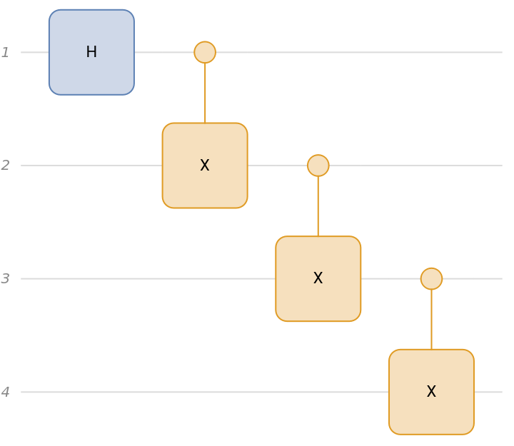
Here we prepare a list of quantum operations or quantum gates.
In[]:=
ghzCircuitoper={QuantumOperator["H"],QuantumOperator["CX",{1,2}],QuantumOperator["CX",{2,3}],QuantumOperator["CX",{3,4}]};
In[]:=
ghzCircuit=QuantumCircuitOperator[ghzCircuitoper];ghzCircuit["Diagram"]
Out[]=
In[]:=
stepsghz=ComposeList[ghzCircuitoper,QuantumState[{"Register",4}]];
The operation or effect of each gate is summarized in a table below -
In[]:=
Grid[Transpose[{Style[#,Bold]&/@{"Initial state","After 1st Hadamard","After 1st CNOT","After 2nd CNOT","After third CNOT"},#["Formula"]&/@stepsghz[[;;-1]]}],Frame->All]
Out[]=
Initial state | |0000〉 |
After 1st Hadamard | 1 2 1 2 |
After 1st CNOT | 1 2 1 2 |
After 2nd CNOT | 1 2 1 2 |
After third CNOT | 1 2 1 2 |
Now we are interested in getting entropy for different partitions of the system. In order to do that, we calculate the Von-Neumann entropy for the reduced density matrices for such partitions.
In[]:=
densityTrace[m_]:=Module[{λ,S,d},{λ,S}=Eigensystem[m];S=Transpose[S];d=Diagonal[Inverse[S].m.S];Total@MapThread[If[#1==0,0,#1 Log[#2]]&,{d,λ}]]
Let’s interpret what we see for different entropy calculations. Here, stepsghz[[n]] represents the n’th state of the quantum circuit. We take different combinations of qubits (three at a time), that will get traced out.
For the first entropy calculation, we took the input state of the circuit. It is 0 for all combinations. This means that none of the qubits are entangled yet.
In[]:=
#->densityTrace@Normal[QuantumPartialTrace[stepsghz[[1]],#]["DensityMatrix"]]&/@Select[Union[Sort/@Tuples[Range[4],3]],DuplicateFreeQ[#]&]
Out[]=
{{1,2,3}0,{1,2,4}0,{1,3,4}0,{2,3,4}0}
In the second entropy calculation, we took the second output state of the circuit, after the Hadamard gate. Again, all entropies are 0. No entanglement still.
In[]:=
#->densityTrace@Normal[QuantumPartialTrace[stepsghz[[2]],#]["DensityMatrix"]]&/@Select[Union[Sort/@Tuples[Range[4],3]],DuplicateFreeQ[#]&]
Out[]=
{{1,2,3}0,{1,2,4}0,{1,3,4}0,{2,3,4}0}
Things start to get interesting when we look at the state after the first CNOT gate . Now we see that the entropy is zero when qubits 1, 2, 3 and 1, 2, 4 are traced out . That means that 3 and 4 are in "0" state with certainty . 1 and 2 have been entangled .
In[]:=
#->densityTrace@Normal[QuantumPartialTrace[stepsghz[[3]],#]["DensityMatrix"]]&/@Select[Union[Sort/@Tuples[Range[4],3]],DuplicateFreeQ[#]&]
Out[]=
{{1,2,3}0,{1,2,4}0,{1,3,4}-Log[2],{2,3,4}-Log[2]}
Similarly, after second gate, we see that entropy is zero only when qubits 1,2,3 are traced out, meaning only qubit 4 is in 0 state now. Finally, for the last step, none of the entropies is 0, so all qubits are entangled.
In[]:=
#->densityTrace@Normal[QuantumPartialTrace[stepsghz[[4]],#]["DensityMatrix"]]&/@Select[Union[Sort/@Tuples[Range[4],3]],DuplicateFreeQ[#]&]
Out[]=
{{1,2,3}0,{1,2,4}-Log[2],{1,3,4}-Log[2],{2,3,4}-Log[2]}
In[]:=
#->densityTrace@Normal[QuantumPartialTrace[stepsghz[[5]],#]["DensityMatrix"]]&/@Select[Union[Sort/@Tuples[Range[4],3]],DuplicateFreeQ[#]&]
Out[]=
{{1,2,3}-Log[2],{1,2,4}-Log[2],{1,3,4}-Log[2],{2,3,4}-Log[2]}
In[]:=
list1=Style[#,Bold]&/@{"Initial state","After 1st Hadamard","After 1st CNOT","After 2nd CNOT","After third CNOT"}
Finally we formulate our results. The second column of the table describes the state after every quantum gate. The third column denotes the entanglement entropy for different partitions of the system. The third column contains the inference we draw from different entanglement entropies.
So this analysis is telling us that the entanglement is spreading in the GHZ circuit with each CNOT gate application. After the next Bell state circuit, we will see how this entanglement spreading can be captured by branchial graphs.
Another GHZ like circuit
Another GHZ like circuit
Here, we are looking at a different circuit in detail just like the GHZ circuit above. We show here the diagram and output states after each gate in the circuit. This section serves as an additional technical exercise to explore entanglement spreading in other circuits.
We now look at the multiway graphs for the GHZ circuit and the circuit just above. We note that there is more branching for the second circuit with more Hadamard gate.
We do a similar analysis that we did above for GHZ circuits. These calculations trace out different combinations of 3 and 2 qubits for the circuit. Here, we just show that the entropy spreading is different.
Finally we formulate our results . The second column of the table describes the state after every quantum gate . The third column denotes the entanglement entropy for different partitions of the system . The third column contains the inference we draw from different entanglement entropies . The fourth column shows the entanglement entropy for when we partition the system in 2 and 2 qubits.
It is important to note here that the entanglement entropy is same for both the circuits, however the nature of how entanglement spreads is different .
Another important message is that we get Log[4] entanglement entropy when we partition the 4 qubit system to 2+2 qubit system. This shows that the number of common ancestors and how far away they are on a multiway graph affects the entanglement entropy. This indicates that we can indeed study these entanglement entropies and spreading with multiway graphs and branchial graphs.
Another important message is that we get Log[4] entanglement entropy when we partition the 4 qubit system to 2+2 qubit system. This shows that the number of common ancestors and how far away they are on a multiway graph affects the entanglement entropy. This indicates that we can indeed study these entanglement entropies and spreading with multiway graphs and branchial graphs.
Branchial graphs
Branchial graphs
The concept of branchial graphs in the multiway system denote the adjacency of different "states" on the multiway graph . In this approach, two branches of evolution at a particular time are "adjacent" if they share an immediate ancestor in their multiway graph .
Here we define different levels of branchial graphs . For level 1, we join the nodes or states of the multiway system if they share a common ancestor . For level 2 branchial graph, we join nodes such that at least for one of them, the common ancestor two steps away . For level n, the nodes will be connected if for at least one of them the common ancestor is n steps away .
Here we define different levels of branchial graphs . For level 1, we join the nodes or states of the multiway system if they share a common ancestor . For level 2 branchial graph, we join nodes such that at least for one of them, the common ancestor two steps away . For level n, the nodes will be connected if for at least one of them the common ancestor is n steps away .
Print multiway graph for GHZ circuit again-
Here we find vertices where the number of outgoing edges are two or more-
In[]:=
For each branch, there will be one branchial graph per level .
Here we see that the higher order branchial graphs become more connected, representing the entanglement spreading in the quantum circuit. Just like having a common ancestor denotes entanglement in the multiway graph, now tracing ancestry several steps back is key to entanglement spreading in the circuit.
Conclusion
Conclusion
Acknowledgement
Acknowledgement
Random state- Appendix 1
Random state- Appendix 1
Here we confirm that our method of calculating entropy matches with the built-in function “quantumEntanglementMontone”-
Branchial graphs- Appendix 2
Branchial graphs- Appendix 2
This method generates branchial graphs using For loops, which are computationally expensive. Nevertheless, I am including all the things that are not efficient and approaches that don’t work in the appendices.
Here, we generate the graph for the GHZ circuit-
The concept of branchial graphs in the multiway system denote the adjacency of different “states” on the multiway graph. In this approach, two branches of evolution at a particular time are “adjacent” if they share an immediate ancestor in their multiway graph.
Here we define different levels of branchial graphs. For level 1, we join the nodes or states of the multiway system if they share a common ancestor. For level 2 branchial graph, we join nodes such that at least for one of them, the common ancestor two steps away. For level n, the nodes will be connected if for at least one of them the common ancestor is n steps away.
Here we show some examples. This is written using for loops. In the next section, the generation will be programmatically better, thanks to code written by Mano.
For level 1 branchial structure , we find and connect nodes that have one ancestor common
For level 2 Branchial graph, we connect nodes that have a common ancestor at least two steps away.
Same story for level 3 branchial graphs-
Stuff that does not work- Appendix 3
Stuff that does not work- Appendix 3
This method doesn’t work because some eigenvalues of the reduced density matrix are zero. This is why in the sections above, we have only picked the non-zero eigenvalues in the trace.
We now Calculate the entanglement entropy at each step, partitioning the system symmetrically .
We loop over different quantum states produced after each gate, as listed in the table above and calculate density matrix for each state -
We loop over different quantum states produced after each gate, as listed in the table above and calculate density matrix for each state -
We rinse and repeat now - we calculate the reduced density matrices, by tracing out all different qubits . However, we will not repeat the exact procedure of getting the reduced density matrix in the entanglement entropy sub - section . The reason for not repeating the method is that for higher dimensional quantum systems, the reduced density matrices will often have eigenvalues that are 0. So we cherry-pick only the non-zero eigenvalues, meaning the sum of the log of non-zero eigenvalues of the partial trace. I have written this approach here that does NOT work-
CITE THIS NOTEBOOK
CITE THIS NOTEBOOK
Entanglement spreading in quantum circuits, multiway graphs, and branchial graphs
by Shraddha Agrawal
Wolfram Community, STAFF PICKS, Jan 16, 2025
https://community.wolfram.com/groups/-/m/t/3357884
by Shraddha Agrawal
Wolfram Community, STAFF PICKS, Jan 16, 2025
https://community.wolfram.com/groups/-/m/t/3357884