Visit the documentation page with more details and full list of examples here: https://resources.wolframcloud.com/FunctionRepository/resources/LagrangePointData
◼
Computations are done in a coordinate system that rotates with the two primary bodies as they orbit.
◼
In the coordinate system used, the origin is at the center of mass of the system and the orbiting bodies orbit in the - plane with the -axis perpendicular to that plane.
x
y
z
◼
The positive -direction is in the direction of the smaller mass.
x
◼
The positive -direction follows a right-hand rule convention.
y
◼
The gravitational effective potential includes terms for the masses of the two bodies in addition to a centripetal term due to the orbital motion.
◼
The distance between the two bodies changes with time, scaling the numbers accordingly.
◼
For a given date, the gravitational effective potential assumes a circular orbit of and using the distance on that date () as the distance between the bodies.
entity
1
entity
2
a
Examples
Examples
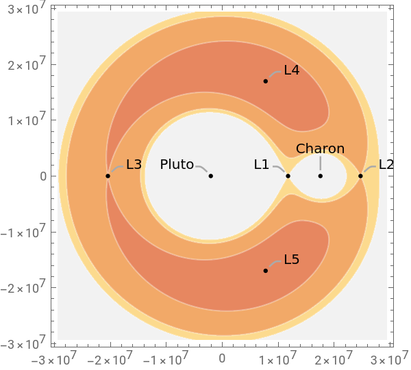
Create a contour plot of the gravitational effective potential with distances:
In[]:=
Grid,,{"ContourPlot","Distances"},ImageSize->300,TargetUnits->"Kilometers"
Out[]=
Create a 3D surface plot of the gravitational effective potential:
In[]:=
Out[]=

Create a 3D contour plot of the gravitational effective potential:
In[]:=
Out[]=

Emphasize the area around the secondary mass as 3D contours:
In[]:=
Out[]=

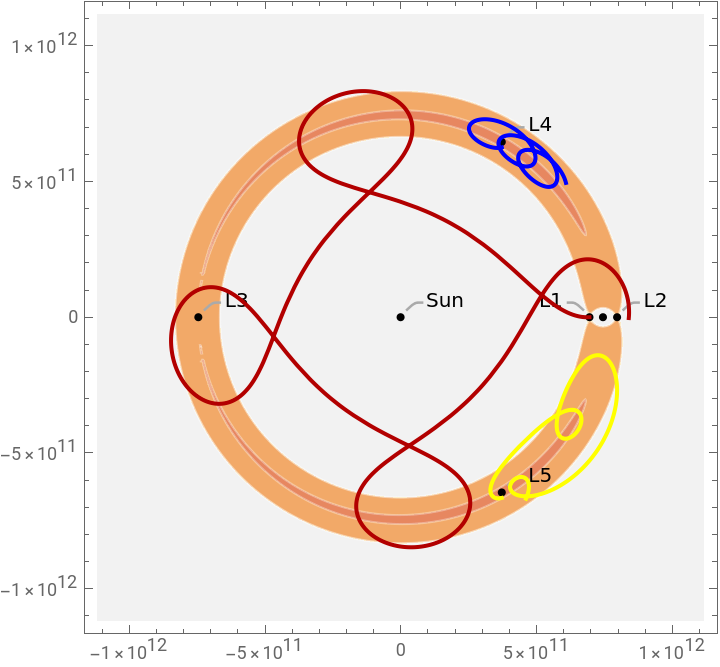
Explore the Lagrange points of the Sun-Jupiter system:
In[]:=
{ω,V,L1,L4,L5,cp}=Flatten{{QuantityMagnitude[#[[1]]],#[[2]][x[t],y[t],z[t]],QuantityMagnitude[#[[3]]],QuantityMagnitude[#[[4]]],QuantityMagnitude[#[[5]]]}&@Lookup[#[[1]],{"ω","NondimensionalizedPotential","L1Position","L4Position","L5Position"}],#[[2]]}&@,,{"GravitationalEffectivePotentialData","ContourPlot"},1/.z[t]->0;
Solve the equations of motion for a particle starting at the L1 point and moving in the --direction and --direction over a period of about 31 years (1,000,000,000 seconds):
x
y
In[]:=
L1sols=NDSolve[{x''[t]-2ωy'[t]==-D[V,x[t]],y''[t]+2ωx'[t]==-D[V,y[t]],x'[0]==-5000.,y'[0]==-300.,x[0]==L1[[1]],y[0]==L1[[2]],z[0]==L1[[3]]},{x,y},{t,0,1000000000}];
Solve the equations of motion for particle starting near the L4 and L5 points with different initial velocities:
In[]:=
L4sols=NDSolve[{x''[t]-2ωy'[t]==-D[V,x[t]],y''[t]+2ωx'[t]==-D[V,y[t]],x'[0]==-1000.,y'[0]==-300.,x[0]==L4[[1]],y[0]==L4[[2]]-20000000000,z[0]==L4[[3]]},{x,y},{t,0,1000000000}];
In[]:=
L5sols=NDSolve[{x''[t]-2ωy'[t]==-D[V,x[t]],y''[t]+2ωx'[t]==-D[V,y[t]],x'[0]==-1000.,y'[0]==-300.,x[0]==L5[[1]],y[0]==L5[[2]]-20000000000,z[0]==L5[[3]]},{x,y},{t,0,1000000000}];
In[]:=
L1path=ParametricPlot[Evaluate[{x[t],y[t]}/.L1sols],{t,0,1000000000},PlotStyle->Darker[Red,.3]];
In[]:=
L4path=ParametricPlot[Evaluate[{x[t],y[t]}/.L4sols],{t,0,1000000000},PlotStyle->Blue];
In[]:=
L5path=ParametricPlot[Evaluate[{x[t],y[t]}/.L5sols],{t,0,1000000000},PlotStyle->Yellow];
In[]:=
Show[{cp,L1path,L4path,L5path},PlotRange->All]
Out[]=
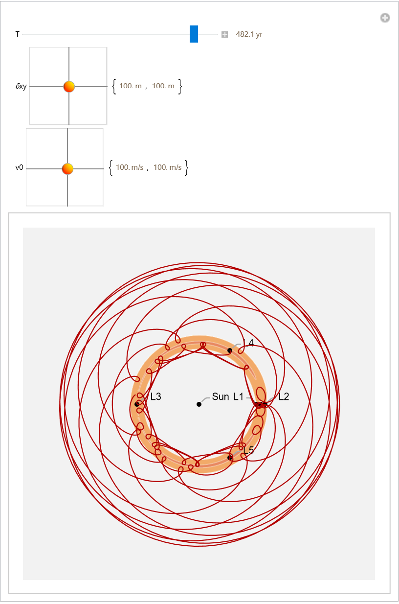
Explore the space of possible orbits of a test particle starting near L4:
In[]:=
Manipulate[Module[{sol,L4=Most[L4]},sol=NDSolve[{x''[t]-2ωy'[t]==-D[V,x[t]],y''[t]+2ωx'[t]==-D[V,y[t]],x'[0]==v0[[1]],y'[0]==v0[[2]],x[0]==L4[[1]]+δxy[[1]],y[0]==L4[[2]]+δxy[[2]]},{x,y},{t,0,10^T}];Show[{cp,ParametricPlot[Evaluate[({x[t],y[t]})/.sol],{t,0,10^T},PlotStyle->Directive[Darker[Red,.3],Thickness[0.003]],Frame->True,Axes->False]},PlotRangePadding->1*^12,Frame->False,Axes->False,Background->GrayLevel[.95]]],Row[{Control[{{T,10.2,"T"},3,11}]," ",Dynamic[Quantity[Round[10^T/3.28725`*^7,0.1],"Years"]]}],Row[{Control[{{δxy,{100,100}},10^6{-1,-1},10^6{1,1}}]," ",Dynamic[Quantity[Round[δxy,0.1],"Meters"]]}],Row[{Control[{{v0,{575,-300}},10^4{-1,-1},10^4{1,1}}]," ",Dynamic[Quantity[Round[δxy,0.1],"Meters"/"Seconds"]]}],SynchronousUpdating->False]
Out[]=
CITE THIS NOTEBOOK
CITE THIS NOTEBOOK
LagrangePointData: Compute properties for the Lagrange points of two orbiting astronomical bodies
by Jeff Bryant
Wolfram Community, STAFF PICKS, December 15, 2023
https://community.wolfram.com/groups/-/m/t/3085142
by Jeff Bryant
Wolfram Community, STAFF PICKS, December 15, 2023
https://community.wolfram.com/groups/-/m/t/3085142