The current essay presents a method for interpolation of smooth functions on the surface of a sphere. Given the value of the function at three points on the sphere, the method estimates its value at some other point, and the error of this estimate is roughly proportional to the square of the distance between the points. One interpretation of the method is that it takes the cross-section of the sphere by the plane that goes through the three reference points and then uses bilinear interpolation on that plane; effectively, it approximates small spherical triangles as being flat. Another interpretation is that it is a scaled-down version of trilinear interpolation in which the gradient lies in the plane formed by the three points. Yet another interpolation is that the method approximates functions as a sum of the spherical harmonics ,,,; being the eigenfunctions of Laplace’s operator, spherical harmonics are smooth, well-behaved, and “meaningful”. To assess the effectiveness of the method, it is compared against Shepard interpolation and the Wolfram Language default interpolation (bilinear interpolation with and as the independent variables). The presented method of interpolation was judged to be superior in terms of accuracy for interpolation on small distances. While the WL default interpolation does pretty well near the equator, it is unusable near the poles because of the singularity in spherical coordinates. The error of the Shepard interpolation grows linearly with distance, which makes it significantly less accurate on small distances. In terms of computation time, the presented method is similar to Shepard interpolation. It evaluates exactly to the sampled values at the reference points.
Y
0,0
Y
1,-1
Y
1,0
Y
1,1
ϕ
θ
Intuitive motivation
Intuitive motivation
Interpolation on a sphere is a nontrivial problem. One reason for that is curvature. On a plane, we could just write , where is the function being interpolated, is the position vector of a point, and the scalar and the 2-dimensional vector are constants. Knowing the values ,, of at any three given points ,, would suffice to find and . And knowing the values of and , one can compute the estimated value for any point . Simple! Wouldn’t it be nice if we could do something like this on a sphere? One option is to simply take , where and are the longitude and latitude, respectively. But this approach completely breaks down near the poles because of the singularity in spherical coordinates. It would be nice to have a more “spherically-compatible” way of generalizing bilinear interpolation. Imagine a smooth function defined on the surface of the unit sphere; in spherical coordinates, . We are given three points in three-dimensional space with radius-vectors ,, that lie on the unit sphere (in the figure below, they are connected into a triangle), and the values =ψ[], =ψ[], =ψ[]. The task is to estimate at some point which lies somewhere in-between ,,:
ψ[r]=+v·r
ψ
0
ψ
r=(x,y)
ψ
0
v
ψ
1
ψ
2
ψ
3
ψ
r
1
r
2
r
3
ψ
0
v
ψ
0
v
ψ[R]
R
ψ=+aϕ+bθ
ψ
0
ϕ
θ
ψ
ψ=ψ[ϕ,θ]
r
1
r
2
r
3
ψ
1
r
1
ψ
2
r
2
ψ
3
r
3
ψ[R]
R
r
1
r
2
r
3
Out[]=

The three points form a so-called “spherical triangle”, which is concave. But provided that the triangle is small, it is a good approximation to neglect its curvature:
Out[]=
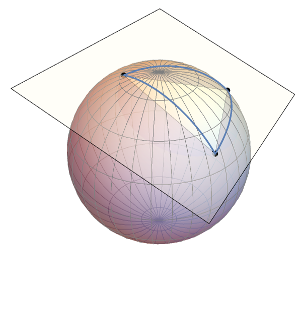
By taking the cross-section of the sphere by a plane that passes through the three reference points, we effectively reduce the problem to interpolation on a plane. There is a certain function whose value is known at three points ,,, and we want to find its value at . While is only defined on the surface of the sphere and not in the entire three-dimensional space, we can imagine a new function that is defined on the ,, plane. is also unknown, but it allows us to use the good old plane interpolation. We can use the model [r]=+v·r, where the vector is a three-dimensional vector that lies in the ,, plane, in analogy with how in bilinear interpolation. (Important note here: “ lies in the plane” is used not in the linear algebra meaning but rather, if the “tail” of was brought to some point in the plane, then the “head” of would also be in the plane.) As an estimate for , we would have [], where is the orthogonal projection of onto the plane (see figure below). By the definition of orthogonal projection, -R is orthogonal to any vector in the plane, and since the vector lies in the plane, . Hence, the estimate for is just +v·R, where and are constants chosen such that +v·=, +v·=, +v·=, and lies in the ,, plane.
ψ
r
1
r
2
r
3
R
ψ
*
ψ
r
1
r
2
r
3
*
ψ
*
ψ
ψ
0
v
r
1
r
2
r
3
v∈
2
v
v
v
ψ[R]
*
ψ
*
R
*
R
R
*
R
v
v·=v·R
*
R
ψ[R]
ψ
0
ψ
0
v
ψ
0
r
1
ψ
1
ψ
0
r
2
ψ
2
ψ
0
r
3
ψ
3
v
r
1
r
2
r
3
Out[]=
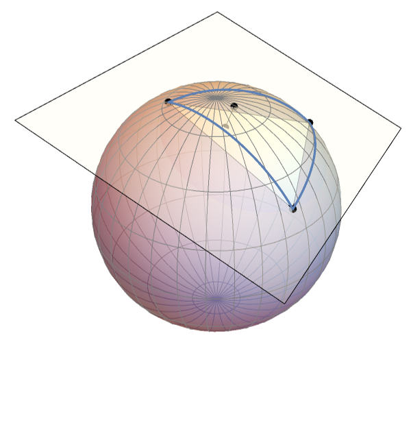
Here is another interpretation. Suppose we “upgrade” from the surface of the sphere to the entire space . We won’t bother about what values has elsewhere from the unit sphere, just demand that remains smooth. Now, we have the problem of interpolating a function in three-dimensional space, and a good candidate is the trilinear interpolation +v·r. Knowing the value of at just three points isn’t enough to find the constants ,v, since now has 3 components and constitutes an additional degree of freedom. The best we can do is to find the “in-plane” component of . Since nothing can be deduced about the perpendicular component of , it is a natural choice to set to it to zero. So again, we have the model , where is a vector that lies in the ,, plane.
ψ
3
ψ
ψ
ψ
0
ψ
ψ
0
v
ψ
0
v
v
ψ=+v·r
ψ
0
v
r
1
r
2
r
3
Out[]=

Here is yet another interpretation (this is the last one). The problem of interpolation can be re-formulated as follows: given the value of the function at three points, estimate the value of the function everywhere else on the sphere. Sphere is symmetric, so correspondingly, any sensible interpolation method should be based on geometrically meaningful things. For example, , where is longitude and is latitude, is not a sensible interpolation because the result it gives depends on which points we choose to be the poles, which is completely arbitrary. A model of the form , however, is completely sensible; there is no “preferred direction” or any other arbitrary things built into it. Moreover, also happens to be a sum of spherical harmonics: for certain ’s. The fact that the spherical harmonics are eigenfunctions of the Laplace’s operator makes them “very meaningful” and guarantees that they are smooth and well-behaved. There are, of course, many other geometrically meaningful models, but this one is among the first that come to mind. Below is an illustration of this interpretation, with color corresponding to the value of . From this picture it can be seen that the interpretation is based around this “kids’ rainbow ball” basis. Notice that the color does not change as we go in the direction perpendicular to the plane of the three points, reflecting the fact that lies in the plane:
ψ
ψ[ϕ,θ]=+aϕ+bθ
ψ
0
ϕ
θ
ψ=+v·r
ψ
0
ψ=+++
ψ
0
v
1
r
1
v
2
r
2
v
3
r
3
ψ=+++
0,0
Y
0,0
1,-1
Y
1,-1
1,0
Y
1,0
1,1
Y
1,1
ψ
v
Out[]=

Code used to generate the figures
Code used to generate the figures
Quantitative analysis
Quantitative analysis
Numeric test
Numeric test
5
.Repeat the first four steps a large number of times.
6
.Make a histogram of the results.
Why Shepard interpolation has linear error
Why Shepard interpolation has linear error
How the Wolfram Language default interpolation can give unrealistically large estimates
How the Wolfram Language default interpolation can give unrealistically large estimates
Code used to generate the sphere figure
Code used to generate the sphere figure
Coming back to cutting plane interpolation
Coming back to cutting plane interpolation
Code used for the test
Code used for the test