Abstract: The trajectories of planets in a solar system can be calculated from the masses of planets and the distances between them. Though the gravitational formula is simple, the orbits of celestial bodies can be quite complex, as they continuously move due to the force of gravity. The three-body problem is the problem of solving for the motion over time of three celestial bodies, which can be simulated relatively accurately by computers in simulations called n-body simulations. N-body simulations implement the gravitational formula in short increments and interpolate for values in between. In the case of planets with random parameters placed nearby each other in space, their motions are often visually much more chaotic than the circular, regular motions of our solar system. However, if the parameters are such that one object is much more massive than the other celestial bodies, such as a star with planets, then the orbits will be close to the shapes of conic sections, like in our solar system.
Introduction
Introduction
Though there are many parameters to analyze, the aim of my project is to analyze the data from n-body simulations using 3D graphs, as well as visualize the planets’ orbits. The function NBodySimulation was used to get data for the positions and velocities of the planets.
Developing the Orbit Visualization
Developing the Orbit Visualization
An introduction of the case
An introduction of the case
The first step is to create a visualization of a planet orbiting around a star in a stable solar system. To do this, the masses, positions, and velocities of the planets were defined, as the function NBodySimulation uses these as inputs.
Equations were created for orbital speed and orbital period. These equations give the speed a planet would be travelling at, and the amount of time it would take to complete one revolution around its star, for a star of mass M and distance r from the planet.
Equations were created for orbital speed and orbital period. These equations give the speed a planet would be travelling at, and the amount of time it would take to complete one revolution around its star, for a star of mass M and distance r from the planet.
In[]:=
orbitalSpeed[M_,r_]:=UnitConvertUnitSimplifySqrt*Quantity[M,"Kilograms"]Quantity[r,"AstronomicalUnit"],"AstronomicalUnit/Day"
In[]:=
orbitalPeriod[M_,r_]:=UnitSimplifySqrt(4Pi^2*Quantity[r,"AstronomicalUnit"]^3)*Quantity[M,"Kilograms"]
Next, the positions of the star and planet were defined, with “plaa” being the name of the star, and “neet” being the name of the planet.
In this case, the star is located at the origin in the coordinate plane, and the planet is at 1 astronomical unit away from the star in the x-direction, with an initial velocity in the y-direction.
In this case, the star is located at the origin in the coordinate plane, and the planet is at 1 astronomical unit away from the star in the x-direction, with an initial velocity in the y-direction.
In[]:=
plaaPosition=Table[Quantity[0,"AstronomicalUnit"],3]
Out[]=
,,
In[]:=
neetPosition=Quantity[#,"AstronomicalUnit"]&/@{1,0,0}
Out[]=
,,
Then, velocities were defined such that the star, plaa, initially remains stationary, while the planet’s velocity perpendicular to the gravitational acceleration is enough for it to remain in circular orbit.
In[]:=
plaaVelocity=plaaPosition/Quantity[1,"Day"]
Out[]=
,,
The velocity of the planet, neet, can be approximated by finding its orbital period, subtracting its positions one day apart from each other, and dividing that quantity by one day.
In[]:=
UnitConvert[orbitalPeriod[10^30,1],"Days"]
Out[]=
In[]:=
neetVelocity=Cos[2Pi/515.1],Sin[2Pi/515.1],0-Quantity[1,"Day"]
,,
Out[]=
,,
This could similarly be approximated using the orbitalSpeed function defined earlier.
In[]:=
{Quantity[0,"AstronomicalUnit/Day"],#,Quantity[0,"AstronomicalUnit/Day"]}&[orbitalSpeed[10^30,1]]
Out[]=
,,
The mass of the star is defined here as 10^30 kg, which is about half of the mass of the sun, and the mass of the planet is defined here as 10^25 kg, which is slightly more mass than that of the earth.
In[]:=
orbitSimulateData=NBodySimulation"Newtonian",<|plaa-><|"Mass"->,"Position"->plaaPosition,"Velocity"->plaaVelocity|>,neet-><|"Mass"->,"Position"->neetPosition,"Velocity"->neetVelocity|>|>,Quantity[10,"Years"]
Out[]=
NBodySimulationData
This gives the data for one planet orbiting around a star.
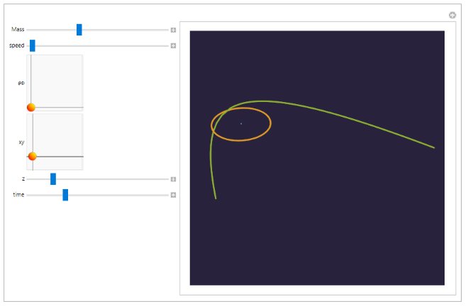
Next, the orbits of two planets around a star were plotted. The user can use the sliders to change the parameters of one of the planets, named “munok”, to observe that its orbit can vary significantly from the near-circular orbit of the other planet. In particular, its orbit will most likely have higher eccentricity, which is the value for how much a conic section, or orbit, varies from being circular.
The incoming planet’s mass, speed, and z-coordinate can each be changed by using the 1-dimensional sliders, while the direction in spherical coordinates (θΦ) and the coordinates on the xy plane can each be changed by using the 2-dimensional sliders.
Visualization of two planets orbiting around a star
Visualization of two planets orbiting around a star
In[]:=
ManipulateParametricPlot3DEvaluateNBodySimulation"Newtonian",<|plaa-><|"Mass"->,"Position"->plaaPosition,"Velocity"->plaaVelocity|>,neet-><|"Mass"->,"Position"->neetPosition,"Velocity"->neetVelocity|>,munok-><|"Mass"->Quantity[Mass*10^23,"Kilograms"],"Position"->Unevaluated[Quantity[#,"AstronomicalUnit"]&/@{First[xy],Last[xy],z}],"Velocity"->Unevaluated[Quantity[#,"AstronomicalUnit/Day"]&/@FromSphericalCoordinates[{speed,First[θΦ],Last[θΦ]}]]|>|>,Quantity[10,"Years"][All,"Position",t],{t,0,time},Background->Hue[0.7,0.44,0.24],Boxed->False,Axes->None,PlotRange->All,{Mass,0.1,10},{speed,0.01,0.03},{θΦ,{0.1,-3.14},{Pi,Pi}},{xy,{-1,-1},{1,1}},{z,-5,5},{time,0.1,3*10^8}
Image of the Manipulate interface, as well as an example. The Manipulate can be run in the downloaded notebook.
Out[]=
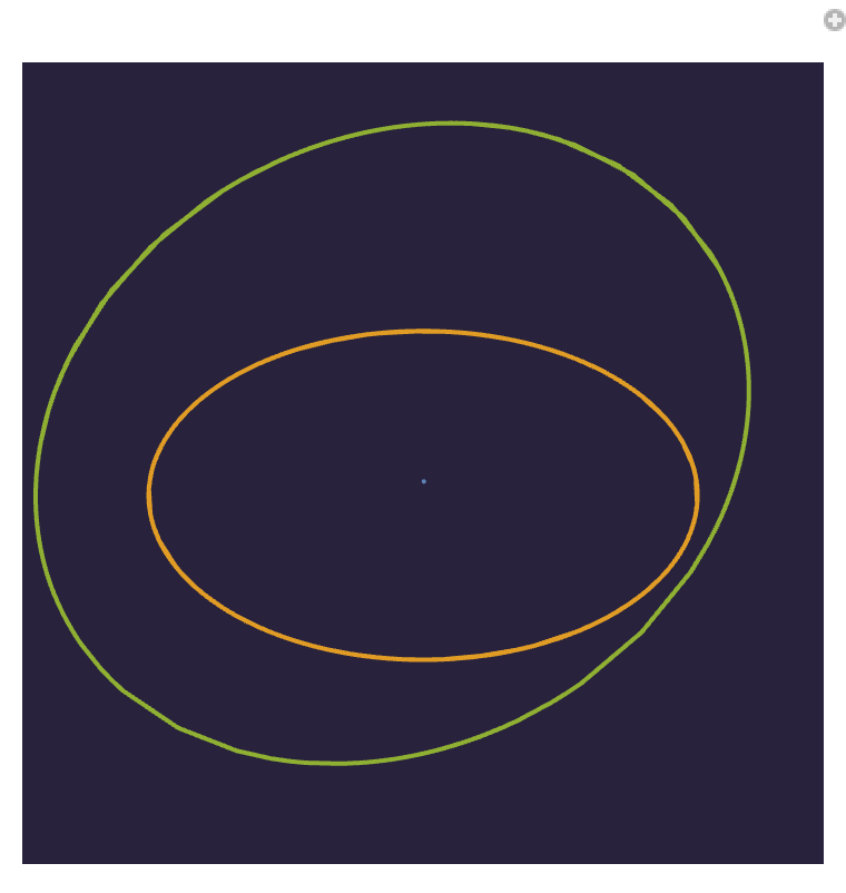
Alternatively, one could visualize the orbits of two stars and a planet, rather than two planets and a star. This would be a binary star system with one planet. In this case, the star and planet are the same as from the previous model, but the incoming planet is instead an incoming star due to its much higher mass.
-A visualization of an interesting case
-A visualization of an interesting case
In[]:=
ManipulateShowParametricPlot3DEvaluateNBodySimulation"Newtonian",<|plaa-><|"Mass"->,"Position"->plaaPosition,"Velocity"->plaaVelocity|>,neet-><|"Mass"->,"Position"->neetPosition,"Velocity"->neetVelocity|>,munok-><|"Mass"->Quantity[Mass1*10^32,"Kilograms"],"Position"->Unevaluated[Quantity[#,"AstronomicalUnit"]&/@{First[xy],Last[xy],z}],"Velocity"->Unevaluated[Quantity[#,"AstronomicalUnit/Day"]&/@FromSphericalCoordinates[{speed,First[θΦ],Last[θΦ]}]]|>|>,Quantity[10,"Years"][All,"Position",t],{t,0,m},Background->Hue[0.7,0.44,0.24],Boxed->False,Axes->None,{Mass1,0.1,10},{speed,0.01,0.03},{θΦ,{0.1,-3.14},{Pi,Pi}},{xy,{-10,-10},{10,10}},{z,-5,5},{m,0.1,3*10^8}
This is an example of what the Manipulate would output, when run on Desktop:
Define the positions of small stars in the background as points with random x- and y- coordinates.
Show a hyperbolic orbit with paths being colored as pink-to-green:
An explanation of the case where I will analyze it
An explanation of the case where I will analyze it
In this case, a planet is in a stable circular orbit around a star, while another planet is placed at a given distance from the star with a given velocity. A list was defined for the eight chosen initial distances, in AU, of 0.3, 0.5, 1.5, 3, 5, 7.5, 10, and 15.
Applying the orbital speed equation to these will give the orbital speed, in astronomical units per day, that a planet in a circular orbit would travel at these distances from the star.
While these are scalar, as they represent speed, NBodySimulation requires velocity, a vector, as input.
Converting the speeds to velocities:
The initial speeds decrease for planets farther away from the star. This is because planets that are farther away experience less gravitational acceleration from their star, so their tangential velocity can be slower to result in a circular orbit.
When a planet is close to a star but orbiting slowly, the acceleration from the gravity of the star will cause the planet’s orbit to become elliptical. However, if a planet is far from a star but orbiting quickly, the acceleration from the gravity of a star will not be enough for the planet’s orbit to become circular, so it will be elliptical in the opposite direction as it would be for a planet that is close to its star and orbiting slowly.
By matching up the eight different speeds with the eight different distances from the star, the data for the sixty-four possibilities could be retrieved using NBodySimulation.
By matching up the eight different speeds with the eight different distances from the star, the data for the sixty-four possibilities could be retrieved using NBodySimulation.
In the two-body problem, which solves for the motion of two celestial bodies, one way to measure whether an object will stay in orbit is the specific orbital energy. When an object is in orbit around another object, its specific orbital energy will be negative. If it has escaped the gravitational influence of its star, then its specific orbital energy will be positive. In this case, the planet has reached escape velocity.
Define a function to receive the data of a planet p’s velocity from an NBodySimulation d at time t:
Define a function for orbital energy:
This takes the inputs of the mass (m), the planet (p), and the NBodySimulation that was run to calculate the data (d).
Getting the data
Getting the data
The following uses orbitalEnergy to calculate the sum of the kinetic and potential energy of each simulation. With this, it can be determined whether the planet will remain in orbit, or leave the solar system.
The data visualization
The data visualization
A table can be made by correlating each energy to the respective initial position and velocity. For example, {3, 7} corresponds to the 3rd position in the list of positions, and the 7th speed in the list of speeds.
Scaled {position, velocity}:
Calculating orbital energy of each simulation:
Next, a function was defined to calculate a planet’s escape velocity:
Then, a function was made to determine whether a planet has reached escape velocity by comparing its velocity at a point in time with its escape velocity based on the mass of the star it is escaping from and the distance the planet is from the star.
For example, note that planet neet is always orbiting its star.
If its orbit was in the shape of an ellipse with higher eccentricity, it would still be orbiting its star.
Then, points were applied the color green if they did not reach escape velocity, and red if they did reach escape velocity, after the simulation had run for 1 million seconds.
The surface of the plot is colored red for higher orbital energies, and colored blue for lower orbital energies. Notice that for higher orbital energies, the planet reached escape velocity. This is because the planets with higher orbital energies are the ones that escaped, since they had enough energy to do so.
The points that are green are in stable orbit, as their orbits are elliptical.
The points that are green are in stable orbit, as their orbits are elliptical.
Future Work
Future Work
In the future, I would like to implement things such as analyzing more complex cases of the three-body problem, as well as visual decorations such as placing spheres at the positions of the planets and having a background sphere of stars that shifts for different viewpoints. I would also like to be able to measure the eccentricity of the orbit by calculating the conic section that the orbit is most similar to, and calculating the eccentricity from that.
Conclusion
Conclusion
In conclusion, this project was able to visualize the orbits of planets on a parametric plot, as well as analyze whether they had reached escape velocity. The effects of the planet’s distance from its star and the planet’s tangential velocity were explored in order to show what factors would result in a stable orbit. An interface was made which displays the paths of the planets based on the inverse square law. Through this, the user can change the parameters to observe that planets orbit in conic sections in a system with one star, and follow more complex paths for a system with two or more stars.
Acknowledgements
Acknowledgements
I would like to thank my mentor, Yana Outkin, for helping me through this project and providing guidance! I would also like to thank Macy Levin for her help with this project!
The Wolfram Summer Research Program has been amazing this year and I am grateful for the experience!
The Wolfram Summer Research Program has been amazing this year and I am grateful for the experience!
References
References
CITE THIS NOTEBOOK
CITE THIS NOTEBOOK