Computation of Turning Points of a Multi-Valued Function
Authors: Housam Binous and Ahmed Bellagi
Computation of Turning Points of a Multi-Valued Function
Authors: Housam Binous and Ahmed Bellagi
Authors: Housam Binous and Ahmed Bellagi
We propose to find the turning points of a multi-valued function.
This function, obtained by digitizing a fivefold bifurcating curve (see Fig. 5-26 in Ref. 1), represents the non-isothermal effectiveness factor versus the Thiele modulus.
We propose to find the turning points of a multi-valued function.
This function, obtained by digitizing a fivefold bifurcating curve (see Fig. 5-26 in Ref. 1), represents the non-isothermal effectiveness factor versus the Thiele modulus.
References :
1- S. Elnashaie, F. Uhlig and C. Affane, Numerical Techniques for Chemical and Biological Engineers Using MATLAB®, A Simple Bifurcation Approach, Springer, NY, 2007.
2- S. Wagon, Mathematica in action: Problem solving through visualization and computation, 3rd ed. Springer-Verlag, Berlin, 2010.
1- S. Elnashaie, F. Uhlig and C. Affane, Numerical Techniques for Chemical and Biological Engineers Using MATLAB®, A Simple Bifurcation Approach, Springer, NY, 2007.
2- S. Wagon, Mathematica in action: Problem solving through visualization and computation, 3rd ed. Springer-Verlag, Berlin, 2010.
The digitized data
In[]:=
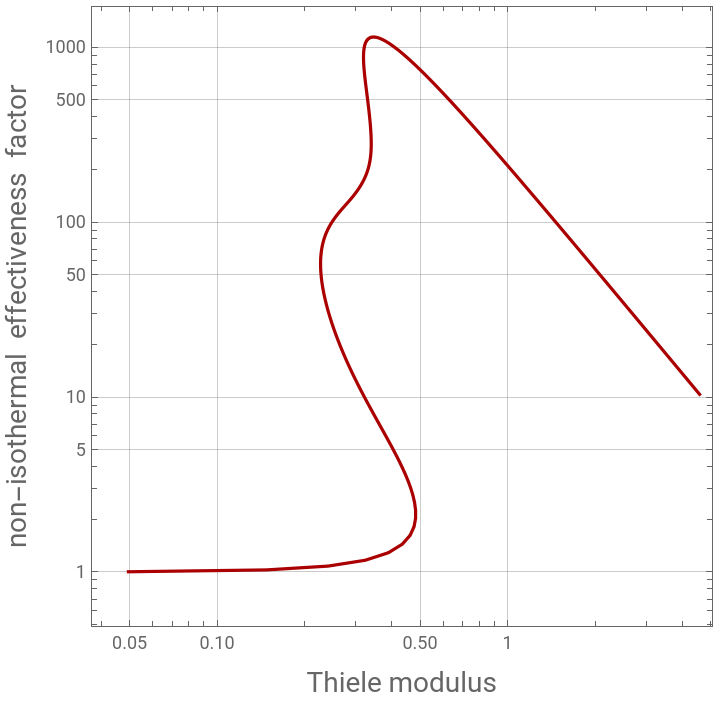
The plot of the function on a Log-Log scale. Clearly, there are several (exactly four) turning points
In[]:=
p1=ListLogLogPlot[data,PlotStyle->{PointSize[0.02],Darker@Red},AspectRatio->1,Frame->True,GridLines->Automatic,Joined->True,FrameLabel->{Style["Thiele modulus",14],Style["non-isothermal effectiveness factor",14]}]
Out[]=
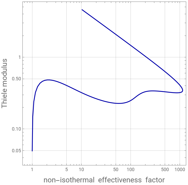
Next we flip the axes and the turning points become the extrema
In[]:=
data1=Table[{data[[i]][[2]],data[[i]][[1]]},{i,1,Length[data]}];
In[]:=
p2=ListLogLogPlot[data1,PlotStyle->{PointSize[0.02],Darker@Blue},AspectRatio->1,Frame->True,GridLines->Automatic,Joined->True,FrameLabel->{Style["non-isothermal effectiveness factor",14],Style["Thiele modulus",14]}]
Out[]=
We compute the derivatives and fetch for the position where the derivatives change sign indicating
the presence of a maximum or a minimum. Details about this approach is available in the textbook by Wagon (Ref. 2).
the presence of a maximum or a minimum. Details about this approach is available in the textbook by Wagon (Ref. 2).
In[]:=
data2=Table[(data1[[i]][[2]]-data1[[i+1]][[2]])/(data1[[i]][[1]]-data1[[i+1]][[1]]),{i,1,200}];
In[]:=
tbl2=Table[data2[[i]],{i,10,150}];
In[]:=
signs=Sign[tbl2];
In[]:=
signs2=Rest[signs]*Rest[RotateRight[signs]];
The positions of the turning points are given below
In[]:=
posns=Position[signs2,-1]
Out[]=
{{2},{45},{88},{131}}
In[]:=
tbl1=Table[data1[[i,2]],{i,10,150}];
In[]:=
turningpoints=tbl1[[Flatten[posns]]]
Out[]=
{0.47648,0.22715,0.339253,0.319161}
In[]:=
tbl2=Table[data1[[i,1]],{i,10,150}];
In[]:=
values=tbl2[[Flatten[posns]]]
Out[]=
{1.81693,54.7168,271.764,854.957}
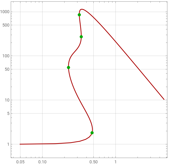
We superpose the plot of the non-isothermal effectiveness factor versus the Thiele modulus
(red curve) and the four turning points (green dots).
(red curve) and the four turning points (green dots).
In[]:=
Show[p1,ListLogLogPlot[Table[{turningpoints[[i]],values[[i]]},{i,1,4}],PlotStyle->{PointSize[0.02],Darker@Green},AspectRatio->1,Frame->True,GridLines->Automatic]]
Out[]=
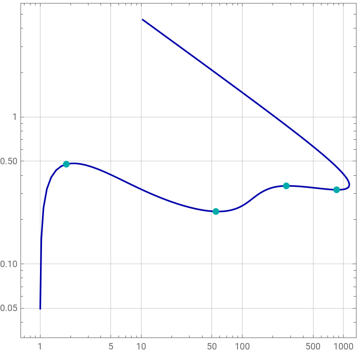
We superpose the flipped plot of the non-isothermal effectiveness factor versus the Thiele modulus
(blue curve) and the four turning points (cyan dots).
(blue curve) and the four turning points (cyan dots).
In[]:=
Show[p2,ListLogLogPlot[Table[{values[[i]],turningpoints[[i]]},{i,1,4}],PlotStyle->{PointSize[0.02],Darker@Cyan},AspectRatio->1,Frame->True,GridLines->Automatic]]
Out[]=