This notebook shows, metaphorically, how to find a 2,000-dimensional needle in a 2,000-dimensional haystack. Finding the needle takes fewer than 160,000 bisections more than 80% of the time.
The algorithm explored here is an abstraction of HPL (human-preference learning, https://openai.com/research/learning-from-human-preferences). The purpose of the abstraction is to estimate how many bisections — binary, subjective, human judgments — would be needed in a real robotic application, and thus to estimate the cost of HPL.
HPL might produce better controllers and at much lower cost than other methods. HPL is cheap at scale: 100,000 judgments might cost $1000, two hours’ time, roughly, for a consulting engineer. Furthermore, subjective human judgment is actually very refined. Almost anyone can tell the difference, at-a-glance, between an elegant gymnastic performance and a merely flawless one. How much does it cost to hand-write a robotic controller that produces elegant, not merely flawless, gymnastics? How about via standard reinforcement learning? How much does it cost to hand-craft a reward function that distinguishes elegant from flawless? If we could instead find such a controller for a few thousand dollars’ worth of human judgments, is that not interesting?
Background and Motivation
Background and Motivation
In a real robotic application, HPL solicits a judgment by showing to the human two performances of two d-dimensional controllers operating the same robot. The human subjectively picks the better of the two performances.
The two controllers are chosen Gaussian-randomly within an appropriately sized d-ball centered at the last best guess at the controller. The algorithm replaces the old best guess with the new best guess centered at a slightly smaller d-ball, then generates two new random controllers and iterates. When the guess is good enough, subjectively, the algorithm halts. This technique is related to evolutionary strategies (https://en.wikipedia.org/wiki/Evolution_strategy).
2,000 dimensions suffice for a robot with 100 degrees of freedom and 20 actuators, if one seeks the LQR matrix (see https://en.wikipedia.org/wiki/Linear%E2%80%93quadratic_regulator). The matrix linearly transforms state delta to actuator forces. State delta is the difference between current state (simulated or real) and desired state, measuring by how much we “miss the mark.”
K
K
If one instead seeks the and design matrices, nearly diagonal in practice, 2,000 dimensions suffice for, say, 1,000 degrees of freedom with 1,000 actuators. Searching for and has order , whereas searching for has order . measures the cost of applying actuators, where is the number of actuators. measures the cost of missing the mark, where is the number of degrees of freedom. and imply via the Riccati equation.
R
Q
R
Q
R+Q
K
R×Q
R
R
Q
Q
R
Q
K
In other work, we found, in fewer than 30 real human judgments, a 16-dimensional LQR controller for balancing an inverted spherical pendulum (https://www.dropbox.com/scl/fi/pqd8b9f3p0q9sclfc76yy/SphericalPendulumIn28TrialsHighRes.mp4?rlkey=w970cjcwyhp76ozjsy6kasgc7&dl=0). This problem is analytically difficult. At the other extreme, the abstract method in this notebook found an oracular optimum in 5,000 dimensions in only 1.3 million judgments.
A limitation of the present work is that it is only demonstrated on a convex benefit function with one global maximum. We believe it will still work when any one of many local maxima is acceptable, but we have not demonstrated so in this notebook.
Problem Statement
Problem Statement
Estimate , the number of binary judgments needed to find a local maximum of some real-valued benefit function. The search depends on a hyperparameter decay, Δ, explained below. We cannot find without specifying Δ and vice versa. and Δ are linked in a way we do not fully understand. However, we can, in practice, find good, paired values of and Δ such that searches succeed most or even all of the time.
N
N
N
N
The benefit function studied in this notebook is convex, i.e., there is only one maximum. Real-world benefit functions may have more than one acceptable local maximum. Therefore, the estimated s in this notebook are conservative. Real-world counts could be many fewer if searches are allowed to find any acceptable local maximum.
N
One simulated judgment
1
.starts with two Gaussian guesses, and , centered at the current best estimate of the target, and within a statistical search radius , the standard deviation of a Gaussian pseudo-random number generator
A
B
y
p
σ
p
2
.consults an oracle for the Euclidean distance from the true target for each of and (in a real-world setting, the true target is not known; instead, a human chooses, subjectively, between the two, and it is this subjective judgment we wish to harvest)
A
B
3
.re-centers the next search at at the closer of and : ←A if is closer to true target, else ←B
A
B
y
p
A
y
p
4
.sets a smaller search radius for the next search (←Δ;Δ<1); this step explains why Δ is called decay: it’s a “shrinkage factor.”
σ
p
σ
p
Definitions
Definitions
A trial is a sequence of judgments. The biggest trial in this notebook is 2,000 dimensions with a maximum "gas-tank" of 160,000 judgments. It can take a couple of minutes to run on one core. We call the maximum number of judgments, say 160,000, a gas tank, because we fail a search when it "runs out of gas," that is, takes more judgments than we are willing to wait for. We express how long we're willing to wait by putting a number like 160,000 in the gas tank.
◼
REMARK: In other work, we ran a C++ version of this code, and found a 5,000-D optimum in 1.3 million judgments out of a gas tank of 100 million. That was the biggest trial we’ve run so far with any software. It succeeded because of an educated guess at the correct Δ. It took about three hours to run on one core. We do not know whether Mathematica can do a trial that big.
In this notebook, we do episodes of 1600 trials in 16 rollouts of 100 trials each. Each rollout tries a different decay Δ, 16 in all. It takes Mathematica about 6 hours on six cores in 64 GB of memory for an episode of 1600 trials at 2,000 dimensions and a gas tank of 160,000. That's about a quarter billion -vectors, or half a trillion Gaussian samples.
2000
Definitions
Definitions
Out[]//TableForm=
Term | Synonym | Description |
episode | 16 rollouts | parallelizable bunch of rollouts |
rollout | 100 trials | parallelizable bunch of trials |
trial | trajectory, trip | non-parallelizable sequence of judgments |
judgment | choice of one of two guesses, A or B | |
guess | a d-vector |
Searching for Best Δ
Searching for Best Δ
We sweep the the decay in an episode, one Δ in each of 16 rollouts, looking for the best Δ for a given and maxIter, the size of the gas tank. For the biggest episode in this notebook, with and , the best Δ is .
Δ
dim
d=2000
gastank=maxIter=160000
0.999919
ld, Number of Leading Nines in Δ
ld, Number of Leading Nines in Δ
ld is defined as .It measures the number of leading nines in the decimal expansion of Δ. ld decreases — moves closer to 0 and further from 1 — as Δ decreases. We use ld in the demonstrations for convenience.
(-(1-Δ))
log
10
ΔFromLd and ldFromΔ convert back and forth between Δ and its number of leading nines.
In[]:=
ClearAll[ldFromΔ,ΔFromLd];;Table[{ld,NumberForm[ΔFromLd[ld],17]},{ld,1,7,1}]//Grid
ldFromΔ
[Δ_]:=-Log10[1.-Δ];ΔFromLd
[lm_]:=1.--lm
10.
Out[]=
1 | 0.9 |
2 | 0.99 |
3 | 0.999 |
4 | 0.9999 |
5 | 0.99999 |
6 | 0.999999 |
7 | 0.9999999 |
How a Trial Dies or Wanders
How a Trial Dies or Wanders
Dying: Δ too Small
Dying: Δ too Small
When Δ is too small, with fewer nines, closer to 0 than to 1, the search radius shrinks too quickly The trial runs out of gas on a falsely positive trail before it gets close to the target. We can guess, ahead of time, that it will run out of gas, and we can cut the trial off early ("We might be going in the right direction, but we don’t have enough gas to find out.”). The point of quitting early is to save wall-clock time. Episodes take hours to run and anything that speeds them up is worth the trouble.
We predict we’ll run out of gas when the distance of the current estimate from the true target is greater than . We predict, right or wrong, that we're not going to get within of the target in more judgments even if we weren't shrinking . We don't have enough gas by an order of magnitude. We call such a trial "dead." This death-prediction formula, , is just a heuristic. We might find a better heuristic by thinking harder or by doing more trial-and-error tuning.
y
p
10×maxIter×
σ
p
σ
p
10×maxIter
σ
p
10×maxIter×
σ
p
However, we have a way to find out whether this heuristic is too aggressive, i.e., kills the trial too early: run some trials with the death-predictor off and compare them to trials with the death-predictor on. If the heuristic is too aggressive, then the success rate will be higher with the predictor off. We call this test process "assessing the death tax" in a section below.
Wandering: Δ too Big
Wandering: Δ too Big
When Δ is too big, we never find the target because our search doesn't shrink quickly enough. Such trials are "wandering." We can't find out about wandering till we actually run out of gas.
Algorithm
Algorithm
We settled on the following algorithm after previous correct but non-performant attempts. This algorithm has been tuned by trial-and-error.
1
.Given dimension , decay , Euclidean-distance tolerance in the unit -ball, current iteration number , current distance from target, and "gas tank" , sample a target -vector from a uniform distribution in the -ball.
d≥2
Δ<1
tol=0.1
d
i
dist
maxIter≥1
d
d
2
.Set ←, the zero vector in dimensions; set ←1, implying that the covariance matrix is the Identity matrix in dimensions, ; and .
y
p
{0}
d
d
σ
p
d
d
dist←0
3
.Reaping the values that are sown in step 10:
4
.Catching the values potentially thrown in steps 5, 6, 7.3, and 8.3:
Do the death and wandering tests early to avoid computing new samples when not necessary.
5
.if , throw , "Dead."
dist>10×maxIter×
σ
p
{,dist,,target,Δ,i}
y
p
σ
p
6
.If , throw , “Wandering.”
i≥maxIter
{,dist,,target,Δ,i}
y
p
σ
p
Generate and test the two points sequentially to avoid computing if is close enough.
B
A
7
.Generate and Test
A
7
.1
.Generate guess normally distributed around center with standard deviation .
A
y
p
σ
p
7
.2
.Calculate Euclidean distance =||-A
d
A
y
p
||
d
L
2
7
.3
.If <tol throw , “Found.”
d
A
{A,,,target,Δ,i}
d
A
σ
p
8
.If not 7.3, Generate and Test
B
8
.1
.Generate guess normally distributed around center with standard deviation .
B
y
p
σ
p
8
.2
.Calculate Euclidean distance =||-B
d
B
y
p
||
d
L
2
8
.3
.If <tol throw , “Found.”
d
B
{B,,,target,Δ,i}
d
B
σ
p
Prepare iteration.
9
.If <, set ←A and , else set ←Band .
d
A
d
B
y
p
dist←
d
A
y
p
dist←
d
B
10
.Set ←Δ,
σ
p
σ
p
i←i+1
11
.Optionally, Sow where it can be Reaped by the caller for logging, debugging, and visualization
{,dist,}
y
p
σ
p
12
.Go to 3
Iterate steps with a fast, functional fold. Fold goes by the Python name reduce or by the C# name Aggregate. Fold revises estimates by internally iterating over updates. Fold is a function of three arguments: (1) a binary function that converts a state and an update into a new state; (2) an initial state value; and (3) a sequence of updates.
311
Fold(binaryFunction,initialState,sequenceOfUpdates)=do{state←binaryFunction(state,update)}foreveryupdateinupdates.
(
1
)In our particular case, we are folding over the binary function seek, whose two inputs are each tuples:
Foldseek,initialState:{=,dist=0,σ=1},updates:Table[{Δ,target,tol,maxIter,i}foriinRange[{1,maxIter}]],=do{{,dist,}←seekstate:{,dist,},update:{Δ,target,tol,maxIter,i}}forifrom1tomaxIter.
y
p
{0}
d
y
p
σ
p
y
p
σ
p
(
2
)This form iteratively replaces the tuple containing the current state estimate with a new tuple, driven by the update tuple, which contains constants and one variable, . We put the constants in the update tuple to avoid pulling them from the global environment. We test whether that choice, which might make a lot of copies of the constants, is too costly below.
{Δ,target,tol,maxIter}
i
Sampling
Sampling
Uniformly in the d-Ball
Uniformly in the -Ball
d
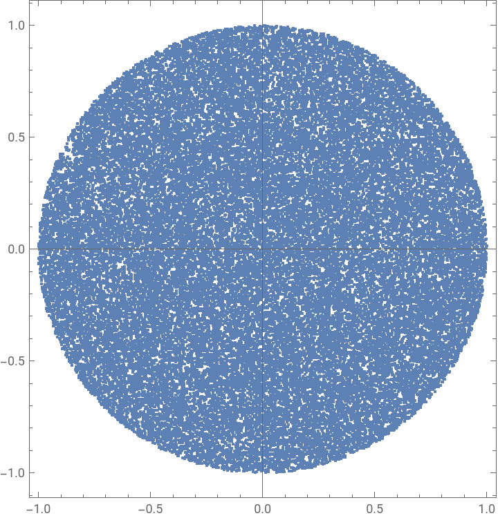
This algorithm exploits Archimedes’s “hat-box” theorem and is the fastest known (see https://community.wolfram.com/groups/-/m/t/3081911). By default, it generates 50,000 uniformly random vectors in 2 dimensions, but it works quickly in any number of dimensions .
>=2
In[]:=
ClearAll[uniformInBall];uniformInDball[n_:50000,d_:2]:=Drop[#,2]&/@Normalize/@RandomVariate[NormalDistribution[],{n,d+2}];
There follows a visual demonstration of uniformity.
In[]:=
ListPlot[uniformInDball[],AspectRatioAutomatic,FrameTrue]
Out[]=
Seeking
Seeking
Bisecting for Δ
Bisecting for Δ
Do One Judgment
Do One Judgment
The following function, doJudgment, performs one judgment. It throws when it dies, or wins within tolerance tol, or runs out of gas wandering. The caller of doJudgment handles all returns in Catch blocks.
Call doJudgment from Fold wrapped in three nested Catches, one for each of “Found,” “Dead,” and “Wandering.” Optionally, doJudgment reaps intermediate results for logging, debugging, and visualization, by setting sow (lower case) to Sow. Sow uses memory, so set sow to Identity for big runs. Likewise, deathTest defaults to True; set it to False to measure the “death tax.” If the death test is too aggressive, you get more wins with deathTest set to False, that is, you will “feel” the “death tax.”
The parameters of doJudgment are split into two lists, the left list holding the prior state, the right list holding inputs for the current call. The output is a new state, so doJudgment meets the requirements for Fold.
Convenient Form for Output
Convenient Form for Output
The following converts outputs from machine-convenient, position-sensitive list form to human-convenient Association form (like dictionary in Python).
Global Constants Timing Test
Global Constants Timing Test
With constants in the update, we don’t need global variables and the code is cleaner. However, it might be expensive to copy constants just for convenience. The following shows that the difference in timing is NOT significant.
Copying Constants into Every Update
The With expression introduces constants into its scope.
Setting Constants Globally
Δ, tar (target), tol (tolerance), maxIter are now global variables; set them directly or in a Block expression.
Visualization Gadget
Visualization Gadget
With the following visualization, experiment interactively with the hyperparameters. Try the various sliders and dimension buttons. Δ is represented by ld, its number of leading nines, smaller for smaller Δ and faster decay; tol and gas tank (number of reps aka maxIter) are logarithmic.
Here is an interactive gadget that does not Sow a visualization. It runs much more quickly than the visualization and confirms it. We did not change the inconsequential call to Reap for fear of breaking the code.
Assessing the Death Tax
Assessing the Death Tax
Trial
Trial
Here is a trial function that does not Sow.
Fast Incremental Statistics
Fast Incremental Statistics
The following are fast incremental statistics in constant memory. See http://vixra.org/abs/1606.0328. We need them to assess success rates and thus the “death tax.”
A bunch of rollouts is an episode. doEpisode depends on trial defined above. It introduces another hyperparameter, maxRol, the number of rollouts in an episode. In this notebook, we leave it at 100.
Do Episode
Do Episode
Quick Test
We now do a fast assessment in two dimensions. Looks like, with the death test off, we don’t get a higher “Found” rate. As expected, we get no dead searches; all failures are wanderers.
Slow Test
With death test off, we get nine more successes, but every failure is a wanderer that must be followed to the bitter end. This takes almost five times longer to run than with death test on. We deem that the death tax is measurable, but probably worth it to save some time. We will miss some searches that will eventually succeed, but not enough to make it worth waiting five times longer. The input cell is commented out, as above, to prevent accidental evaluations. Un-comment and evaluate to reproduce our results.
Here’s the Beef
Here’s the Beef
Getting Ready: 20 Dimensions
Getting Ready: 20 Dimensions
Spot check, on this cheap run, that the death test isn’t doing terrible harm:
Local Stop: 200 Dimensions
Local Stop: 200 Dimensions
Commented out to prevent accidental evaluation. It takes a while to run.
Conclusion: 2000 Dimensions
Conclusion: 2000 Dimensions
CITE THIS NOTEBOOK
CITE THIS NOTEBOOK
How Many Human Preferences for Optimal Control?
by Brian Beckman
Wolfram Community, STAFF PICKS, December 17, 2023
https://community.wolfram.com/groups/-/m/t/3085555
by Brian Beckman
Wolfram Community, STAFF PICKS, December 17, 2023
https://community.wolfram.com/groups/-/m/t/3085555