Chromatographic Reactions of Three Components
Housam Binous
Chromatographic Reactions of Three Components
Housam Binous
Housam Binous
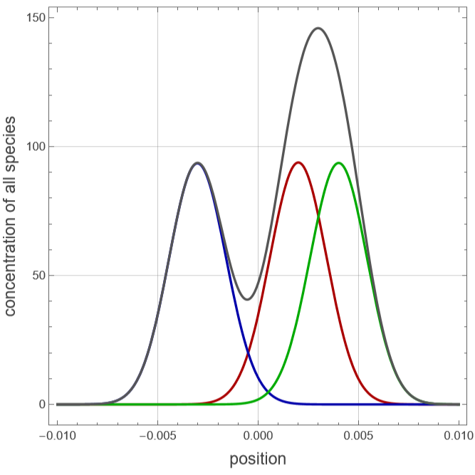
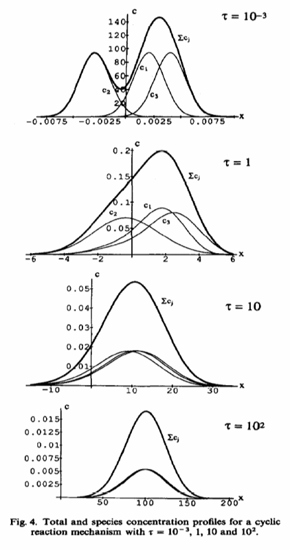
Three species , , and move in an electrostatic, centrifugal, or velocity field and mix according to the cyclic reaction system: . All reaction rate constants are assumed to be equal to =.The three governing equations for the concentrations of the species are=--2++,where } are three permutations of .The boundary and initial conditions are (x,t)=0 and (x,0)=δ(x).All components are assumed to be sufficiently similar to have identical diffusion coefficients The velocities of species , , and are taken to be =0.02cm/s, =-0.03cm/s, and =0.04cm/s.An expression for the reduced first central moment, , the second and third central moments ( and ) were derived in the paper by H. Binous and B. J. McCoy in 1992 (see Ref. 1).These moment expressions are used to construct the concentration profile using the following truncated series of the Gram-Charlier expansion:(x,t)=1+8-126,where =.This notebook shows the concentration profiles of the species , , and at different times. In particular, Fig. 4 of Ref. 1 is reporduced. In accordance with the initial conditions, peaks are very high at small dimensionless time For large values of , all peaks merge into one. Thus, (1) separation of peaks occurs for small ; (2) the species , , and behave as one component for large . For intermediate values of , higher-order terms may be needed to adequately represent the pulse. The concentrations of the species , , and are shown as red, blue, and green peaks, respectively.The gray peak corresponds to (i.e., the concentration of the combined species). This combined concentration exhibits multiple peaks or a broad asymmetric peak for small . This behavior is actually observed in reverse-phase liquid chromatographic separations where one protein can undergo conformational changes and be present in multiple states. Reference:[1] H. Binous and B. J. McCoy, “Chromatographic Reactions of Three Components: Application to Separations,” Chemical Engineering Science, 47(17/18), 1992 pp. 4333–4343. https://doi.org/10.1016/0009-2509(92)85112-O
A
1
A
2
A
3
A
1
k
e
⇆
k
e
A
2
k
e
⇆
k
e
A
3
k
e
⇆
k
e
A
1
k
e
-2
10
-1
s
c
i
A
i
∂
c
i
∂t
D
i
2
∂
c
i
∂
2
x
v
i
∂
c
i
∂x
k
e
c
i
k
e
c
j
k
e
c
m
{i,j,m
{1,2,3}
lim
x±∞
c
j
c
j
1
3
===s.
D
1
D
2
D
3
-5
10
2
cm
A
1
A
2
A
3
v
1
v
2
v
3
μ
1j
μ
2j
μ
3j
c
j
1
3
-
2
X
j
μ
3j
3
X
j
X
j
1.5
2
μ
2j
2π
μ
2j
X
j
x-
μ
1j
2
μ
2j
A
1
A
2
A
3
τ=t.
k
e
τ
τ
A
1
A
2
A
3
τ
τ
A
1
A
2
A
3
3
∑
i=1
c
i
τ
In[]:=
v
1
v
2
v
3
A
1
A
2
A
3
In[]:=
ke=10^-2;(*allreactionrateconstantsareassumedtobeequalto=*)
k
e
-2
10
-1
s
In[]:=
Dif=10^-5;(*Assumeidenticaldiffusioncoefficients===s*)
D
1
D
2
D
3
-5
10
2
cm
In[]:=
(*reducedfirstcentralmoment*)μ[p1,1,t_]:=(2--)(1-Exp[-3ket])/(9ke)+(++)t/3;μ[p1,2,t_]:=(2--)(1-Exp[-3ket])/(9ke)+(++)t/3;μ[p1,3,t_]:=(2--)(1-Exp[-3ket])/(9ke)+(++)t/3;
v
1
v
2
v
3
v
1
v
2
v
3
v
2
v
1
v
3
v
1
v
2
v
3
v
3
v
2
v
1
v
1
v
2
v
3
In[]:=
(*secondandthirdcentralmoments*)
In[]:=
μ[2,1,t_]:=-(2--)^2Exp[-6.ket]/(81ke^2)-2(2^2-^2-^2-2(+-2))tExp[-3ket]/(27ke)+8(^2+^2+^2-(++))Exp[-3.ket]/(81ke^2)+(-4^2-7^2-7^2+4+4+10)/(81.ke^2)+(54Difke+4(^2+^2+^2---))t/(27.ke);μ[2,2,t_]:=-(2--)^2Exp[-6.ket]/(81ke^2)-2(2^2-^2-^2-2(+-2))tExp[-3ket]/(27ke)+8(^2+^2+^2-(++))Exp[-3.ket]/(81ke^2)+(-4^2-7^2-7^2+4+4+10)/(81.ke^2)+(54Difke+4(^2+^2+^2---))t/(27.ke);μ[2,3,t_]:=-(2--)^2Exp[-6.ket]/(81ke^2)-2(2^2-^2-^2-2(+-2))tExp[-3ket]/(27ke)+8(^2+^2+^2-(++))Exp[-3.ket]/(81ke^2)+(-4^2-7^2-7^2+4+4+10)/(81.ke^2)+(54Difke+4(^2+^2+^2---))t/(27.ke);
v
1
v
2
v
3
v
1
v
2
v
3
v
1
v
2
v
1
v
3
v
2
v
3
v
1
v
2
v
3
v
1
v
2
v
1
v
3
v
2
v
3
v
1
v
2
v
3
v
1
v
2
v
1
v
3
v
2
v
3
v
1
v
2
v
3
v
1
v
2
v
1
v
3
v
2
v
3
v
2
v
1
v
3
v
2
v
1
v
3
v
1
v
2
v
2
v
3
v
1
v
3
v
1
v
2
v
3
v
1
v
2
v
1
v
3
v
2
v
3
v
2
v
1
v
3
v
1
v
2
v
2
v
3
v
1
v
3
v
1
v
2
v
3
v
1
v
2
v
1
v
3
v
2
v
3
v
3
v
2
v
1
v
3
v
2
v
1
v
3
v
2
v
1
v
3
v
2
v
1
v
1
v
2
v
3
v
1
v
2
v
1
v
3
v
2
v
3
v
3
v
2
v
1
v
3
v
2
v
1
v
3
v
2
v
1
v
1
v
2
v
3
v
1
v
2
v
1
v
3
v
2
v
3
In[]:=
μ[3,j_,l_,m_,t_]:=-2(2--)^3Exp[-9ket]/(729ke^3)-2(2--)(-4^2+4-4^2+4-4^2+4)+3ket(2^2-2-^2-2-^2+4)Exp[-6ket]/(243ke^3)-(2--)(-2^2+2+16^2+2+16^2-34)+36ket(-^2+-+)+9ke^2t^2(^2-+^2-+^2-)Exp[-3ket]/(243ke^3)+2(2--)(-11^2+11+13^2+11+13^2-37)+9ket(^2--2^2--2^2+5)(729ke^3);
v
j
v
l
v
m
v
j
v
l
v
m
v
j
v
j
v
l
v
l
v
j
v
m
v
m
v
m
v
l
v
j
v
j
v
l
v
l
v
j
v
m
v
m
v
m
v
l
v
j
v
l
v
m
v
j
v
j
v
l
v
l
v
j
v
m
v
m
v
m
v
l
v
j
v
j
v
l
v
l
v
m
v
j
v
m
v
j
v
j
v
l
v
l
v
j
v
m
v
m
v
m
v
l
v
j
v
l
v
m
v
j
v
j
v
l
v
l
v
j
v
m
v
m
v
m
v
l
v
j
v
j
v
l
v
l
v
j
v
m
v
m
v
m
v
l
In[]:=
X
j_
2μ[2,j,t]
;In[]:=
(*concentrationprofileusingthetruncatedseriesexpansion*)
In[]:=
c
j_
X
j
X
j
X
j
2πμ[2,j,t]
;In[]:=
τ=0.001;(*dimensionlesstime*)
In[]:=
plt=PlotEvaluate[x,100τ],[x,100τ],[x,100τ],[x,100τ],{x,-τ10,τ10},PlotRangeAll,FrameTrue,PlotStyle{{Thick,Darker@Red},{Thick,Darker@Blue},{Thick,Darker@Green},{Thick,Darker@Gray}},AxesOrigin{-τ10,0},FrameLabel{Style["position",14],Style["concentration of all species",14]},AspectRatio->1,GridLines->Automatic,ImageSize{400,400}
c
1
c
2
c
3
3
∑
i=1
c
i
Out[]=