Intro
Intro
Definition
Definition
The term "space-filling curve (SFC)" has a strict mathematical definition:
Let ℳ— compact manifold. SFC is continuous map :[0, 1] ℳ such ([0, 1]) ≡ ℳ
Examples are well known: Peano, Hylbert curves etc.
But those constructions on any initial stages are not SFC themselves!
Here we will set a more intuitive and heuristic task:
Construct a curve on the sphere:
- Self-avoiding
- Self-similar
- Continous and closed
- At least intuitively when increasing iterations
approaching each point of the sphere
Examples
Examples
Examples of such designs already exist. They exploit the same idea:
Copying and joining sections of the Peano/Hilbert curve.
1. A seriously developed Google S2 project based on the Hilbert curve.
Copying and joining sections of the Peano/Hilbert curve.
1. A seriously developed Google S2 project based on the Hilbert curve.
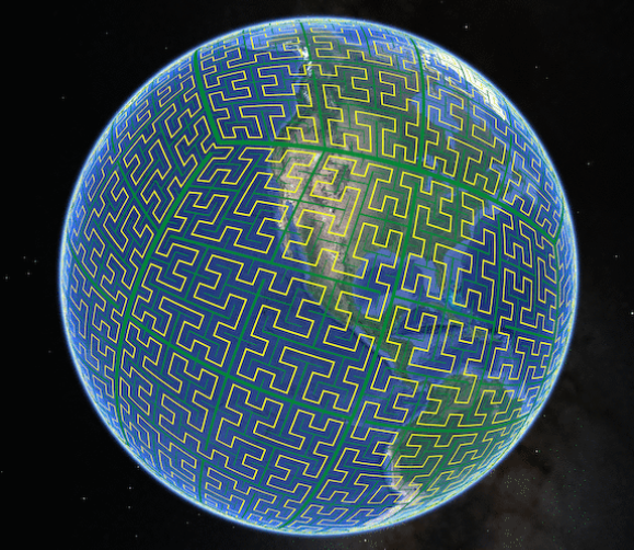
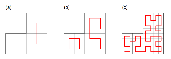
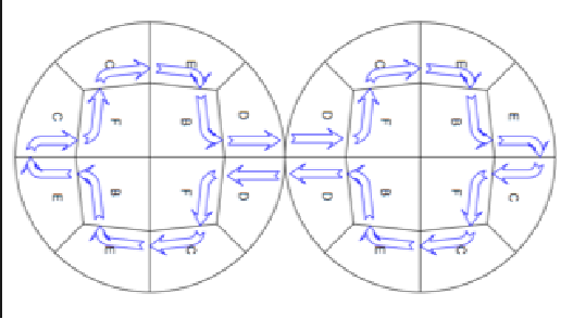
2.Old but detailed work combining the analysis of spherical projectionsand the adaptation of the Hilbert curve to fill the sphere using eight octants. No such example (and no other one I have studied) is Self-similar in the full sense.It is simply the copying and transformation of pieces of known curves.In part II of this project, I will propose a fundamentally different approach.Here we will look at the original version of the sphere filling with coherent sections of self-similar curves,different from all others.
Utilities
Utilities
Our main tool is the parameterization of a large circle (geodesic) on unit sphere,
known as SLERP, here briefly named geo:
known as SLERP, here briefly named geo:
In[]:=
Clear[geo];geo[{p1_?VectorQ,p2_?VectorQ}]:=With[{w=ArcCos@Clip[p1.p2,{-1,1}],u=Normalize[p2-p1(p1.p2)]},p1Cos[w#]+uSin[w#]&];
Graphics utilities
It is known that in Mathematica any curves appear Line or Tube arrays.
I decided to make this process more explicit.
The splineCurve function accepts arguments:
- array of (control) points
- type (1 - plane form, other - 3D form)
- rate: number of subdivisions between control points
- thickness
- spline degree (1 - line)
- closed or not
Clear[ths,g3D,splineCurve];(*Scaledthickness*)ths=2.*10.^Rescale[#,{6,30},{-1.8,-2.1}]&;(*Globalstylecolors*)sCol=Hue[2/3.,1/2.,1/2.];bCol=Hue[2/3.,3/4.,1/6.,1/2.];cCol=Hue[1/8.,3/4.,3/4.];(*General3Dpresentation*)g3D[objs_,size_:200]:=Framed[Graphics3D[{objs},LightingWhite,Boxed->False,SphericalRegion->True,ImageSize->size,ImagePadding->10],RoundingRadius20,Background->bCol,FrameStyle->None];splineCurve[pts_,type_,rate_:5,th_:0.01,sd_:2,cls_:True]:=Block[{bsf=BSplineFunction[pts,SplineDegreesd,SplineClosed->cls],divs=Subdivide[0,1,rate*Length@pts]},If[type==1,{Thickness@th,Line[bsf@#&/@divs]},Tube[Normalize[bsf@#]&/@divs,th]]];
Triangle filled curve
Triangle filled curve
Most examples of space filled curves are based on 4-meshes, although it is known that
that optimal surface models give triangulation.
What if we fill triangle with SFC? Is it possible?
On the Web I found this wonderful example.
I changed the code. Module returns a curve as a list of vertices of a triangular grid.
This is important for the matching with spherical grid.
The curve "enter" triangle in {1, 1} and "exit" from {iters, 1}.
Total number of points is iters (iters+1)/2
In[]:=
Clear[trigPath,trigFCrec];trigFCrec[iters_]:=trigFCrec[iters]=Block[{top={0,1},tr=Function[{x},#+x]&,rotd120={#[[2]],-#[[1]]-#[[2]]}&,rotw60={-#[[2]],#[[1]]+#[[2]]}&,rmc=Reverse@Map[Composition[#1,#2],#3]&,q=Quotient[iters,2],l,s},If[iters<=0,Return[{}]];If[iters==1,Return[{{0,0}}]];If[iters==2,Return[{{0,0},top,{1,0}}]];Join@@If[EvenQ@iters,l=trigFCrec[q];s=trigFCrec[q-1];{rmc[tr[(q-1)top],rotd120,l],tr[qtop]/@l,rmc[tr[{q-1,0}+top],rotw60,s],tr[{q,0}]/@l},l=trigFCrec[q+1];s=trigFCrec[q];{rmc[tr[(q-1)top],rotd120,s],tr[qtop]/@l,rmc[tr[{q,0}],rotw60,s],tr[{q+1,0}]/@s}]];trigPath[num_]:={1,1}+#&/@trigFCrec@num;
In[]:=
ManipulateBlockpts=N{1,1/2},0,
3.
2.#-{1/2,0}&/@(trigPath@n),Graphics[{cCol,splineCurve[pts,1,5,ths@n,sd,False]},ImageSize->200,PlotRange->CoordinateBounds@pts,ImagePadding10,Background->sCol],{{n,10},2,50,1,ControlTypeVerticalSlider,ControlPlacementLeft},{sd,1,3,1,ControlTypeVerticalSlider,ControlPlacementRight},Paneled->False,SaveDefinitionsTrueOut[]=

Plane filled version
Plane filled version
Because the plane is definitely covered by triangles,
we can fill each of them with the obtained above curve,
hoping to fill the plane or its part. But it’s not so simple.
1. The curve runs along the triangle border, so that adjacent fills will stick.
2. I would like to get a closed final curve by filling part of the plane
The first question is simply solved - instead of the triangular network itself, cell centers are taken.
The second question is more complicated. For a small example, we can manually create a matching code
of "enters" and "exits", as done in the next demonstration.
of "enters" and "exits", as done in the next demonstration.
In the general case, the question of closing the path along triangles will be resolved later.
Now let’s build a triangular network on the sphere.
Now let’s build a triangular network on the sphere.
Sphere triangle grid
Sphere triangle grid
Spherical triangle (not necessarily regular, but also not degenerated)
verts is populated with triangle grid of points using a vector algebra.
num - number of points on the side.
Location of vertices in the triangle table:
{{ vert1 = "enter", ..., vert2},
...,
{vert3 = "exit"}}
The code includes correction of "inflation" center area.
The center region is compressed with a parameter g that is visually selected.
Optimal values 0.1 < g < 0.4.
To construct a self-avoiding curve, we use centroids of triangular grid.
Sphere filled curve with triangle cells
Sphere filled curve with triangle cells
Now we can imagine sphere filled with triangle curve.
Split the sphere into 4 quadrants - projections of the tetrahedron’s faces.
Here we also manually configure enter/exit cells connections.
Split the sphere into 4 quadrants - projections of the tetrahedron’s faces.
Here we also manually configure enter/exit cells connections.
Triangulation bypass
Triangulation bypass
In order to efficiently fill with such a curve any triangulation,
we need to connect enters and exits of each triangle correctly.
Perhaps this problem can be formulated using graphs/hypergraphs,
but I used a combinatorial approach, while couldn’t find the correct algorithm myself.
The user of Mathematics SE Misha Lavrov has proposed a universal algorithm, which I use with gratitude here.
Function accepts cyc as already found Hamiltonian cycle of vertices indices (without repeating the first element)
and returns correct closed triangulation bypass cycle.
and returns correct closed triangulation bypass cycle.
Example: Bypass of 5-dypiramid faces
Example: Bypass of 5-dypiramid faces
Collect data:
Select some hamiltonian cycle through faces and look at it:
Now we find a cycle that goes in and out of each faces one time,
with agreement. Make sure that it correctly overrides all faces:
Now we find a cycle that goes in and out of each faces one time,
with agreement. Make sure that it correctly overrides all faces:
Examples
Examples
The result: sphere filled curve
The result: sphere filled curve
There are several ways to triangulate a sphere.
Here we use geodesic polyhedra.
Kardoš (2022) proved that every 3-connected cubic planar graph with faces not
more than 6 vertices have a Hamiltonian cycle.
Because the dual graphs of octahedral geodesic polyhedra have this property,
we can use these polyhedra to construct closed sphere-filled curve.
Let's make it step by step, at the same time go a little deeper into the geometry of polyhedra.
Get polyhedron and it's dual
Find dual graph:
We can be sure that this graph contains a large number of Hamiltonian cycles,
so we can choose a random from some quantity
so we can choose a random from some quantity
Because triangles are different, let’s define the average "density" of the curve
and build a triangular lattice depending on the area of the triangle,
and then we’ll run a closed sphere-filled curve.
Obviously, as the density increases, the curve will approach each point of the sphere evenly.
and build a triangular lattice depending on the area of the triangle,
and then we’ll run a closed sphere-filled curve.
Obviously, as the density increases, the curve will approach each point of the sphere evenly.
Alternative example
Alternative example
We can use a less regular triangulation for example convex hull of Sphere points.
The result will be even more natural:
The result will be even more natural:
CITE THIS NOTEBOOK
CITE THIS NOTEBOOK
Sphere-filling curve 1: generating continuous self-avoiding paths on geodesic polyhedra via dual graph Hamiltonian cycles
by Denis Ivanov
Wolfram Community, STAFF PICKS, September 29, 2026
https://community.wolfram.com/t/28210
by Denis Ivanov
Wolfram Community, STAFF PICKS, September 29, 2026
https://community.wolfram.com/t/28210