Plan for the Talk
Plan for the Talk
I will discuss new features related to the following areas in Version 13.1:
Fractional Calculus
Calculus and Special Functions
Linear Algebra
Documentation
Online Courses
A Recap of Calculus
A Recap of Calculus
Calculus was developed in -century Europe by Isaac Newton and Gottfried Wilhelm Leibniz.
th
17
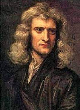
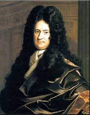
The two fundamental operations of calculus are differentiation and integration:
In[]:=
D[,x]
2
x
Out[]=
2x
In[]:=
Integrate[%,x,GeneratedParametersC]
Out[]=
2
x
1
Integration is essentially the inverse operation of differentiation.
The integral of a function of order n may be regarded as a derivative of order -n.
What is Fractional Calculus?
What is Fractional Calculus?
Fractional calculus generalizes derivatives and integrals to the idea of a “fractional derivative”.
The fractional derivative of a function must have the following properties:
th
α
1. It must be equal to the derivative of the function when α = n is a positive integer.
th
n
2. It must be equal to the repeated integral of the function when α = -n is a negative integer.
th
n
3. Derivatives of other real orders must “interpolate” between the derivatives of integer orders.
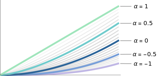
Many definitions of fractional derivatives exist - Riemann-Liouville, Grunwald-Letnikov, Caputo, etc.
We have implemented the Riemann-Liouville and Caputo definitions in Version 13.1.
Riemann-Liouville Derivative
Riemann-Liouville Derivative
FractionalD computes the Riemann-Liouville derivative of a function in 13.1.
The Riemann-Liouville fractional derivative of of order is defined as:
f(x)
α
0
α
D
x
1
Γ(n-α)
n
n
t
x
∫
0
n-α-1
(x-τ)
n=max(0,⌈α⌉)
For example, compute the half-derivative of :
2
x
In[]:=
FractionalD,x,
2
x
1
2
Out[]=
8
3/2
x
3
π
Verify the result using the definition:
In[]:=
Assumingx>0,t
∂
x
x
∫
0
2
t
x-t
Gamma
1
2
Out[]=
8
3/2
x
3
π
Obtain the first derivative:
In[]:=
FractionalDFractionalD,x,,x,
2
x
1
2
1
2
Out[]=
2x
Compute the derivative of arbitrary order α:
In[]:=
FractionalD[,{x,α}]
2
x
Out[]=
2
2-α
x
Gamma[3-α]
Make a table of its values for specific α:
In[]:=
Table%,α,-1,1,
1
2
Out[]=
,,,,2x
3
x
3
16
5/2
x
15
π
2
x
8
3/2
x
3
π
Plot the list of derivatives:
In[]:=
Plot[Evaluate[%],{x,0,1},PlotLegends"Expressions"]
Out[]=


More Examples for FractionalD
More Examples for FractionalD
Compute the fractional derivative of Sin:
In[]:=
FractionalD[Sin[x],{x,α}]
Out[]=
-1+α
2
π
1-α
x
α
2
3
2
α
2
2
x
4
Verify the result for integer orders:
In[]:=
Expand[Table[%,{α,-1,4}]]
Out[]=
{1-Cos[x],Sin[x],Cos[x],-Sin[x],-Cos[x],Sin[x]}
The fractional derivative of a constant is not 0 in general:
In[]:=
FractionalD[c,{x,α}]
Out[]=
c
-α
x
Gamma[1-α]
In[]:=
Table%,α,1,3,
1
2
Out[]=
0,-,0,,0
c
2
π
3/2
x
3c
4
π
5/2
x
The Caputo derivative overcomes this limitation of the Riemann-Liouville derivative.
Caputo Fractional Derivative
Caputo Fractional Derivative
CaputoD computes the Caputo derivative of a function in 13.1.
The Caputo fractional derivative is defined via the formula:
C
0
α
D
x
RL
0
α
D
x
⌈α⌉-1
∑
k=0
k-α
x
Γ(k-α+1)
(k)
f
CaputoD is closely related to FractionalD but it is more suitable for solving practical problems.
Derivative of a Constant
Derivative of a Constant
Laplace Transform
Laplace Transform
The Mittag-Leffler Function
The Mittag-Leffler Function
Special Cases
Special Cases
Several mathematical functions are special cases of MittagLefflerE.
MittagLefflerE itself is a special case of FoxH:
Laplace Transforms
Laplace Transforms
The Laplace transform of MittagLefflerE is an algebraic rational function:
Compute the inverse Laplace transform:
Fractional Differential Equations
Fractional Differential Equations
DSolve can solve any linear fractional differential equation with constant coefficients in 13.1.
Solve following fractional differential equation:
Solve for the Laplace transform:
Find the inverse transform:
Plot the solution:
Systems of Fractional DEs
Systems of Fractional DEs
DSolve can solve any system of linear fractional DEs with constant coefficients in 13.1.
Systems of linear fractional DEs are solved using eigenvalue methods or Laplace transforms.
For example, solve a system of two fractional ODEs in vector form:
Plot the solution:
Parametrically plot the solution:
Singular Solutions from DSolve
Singular Solutions from DSolve
DSolve can compute singular solutions of nonlinear ODEs in 13.1.
The singular solutions are typically either envelope solutions or equilibrium solutions.
For example,
Implicit Differentiation
Implicit Differentiation
ImplicitD can be used to compute the derivatives of implicit functions in 13.1.
Compute the slope of the tangent line to a curve:
Show tangent lines at six points on the curve:
ImplicitD will also help with verifying the results from nonlinear ODEs from DSolve.
Change of Variables in Integrals
Change of Variables in Integrals
IntegrateChangeVariables can be used to apply the method of substitution to integrals.
The new function works on Inactive indefinite integrals, definite integrals and multiple integrals.
Change of Variables in Differential Equations
Change of Variables in Differential Equations
DSolveChangeVariables can be used to apply a change of variables in differential equations.
The new function works for both ordinary differential equations and partial differential equations.
Sums of Residues
Sums of Residues
ResidueSum computes the sum of the residues for a meromorphic function in the complex plane.
This function automates the application of the Cauchy Residue Theorem from complex analysis.
For example,
Integrate the following along the circle with center at the origin and radius 2:
Compute the integral using the residue theorem:
Compare with the result of symbolic integration:
Structured Matrices
Structured Matrices
Six new special, structured matrices have been introduced in Version 13.1.
These matrices return a StructuredArray and are optimized for linear solving, etc.
For example, here is a BlockDiagonalMatrix:
Display the matrix:
Perform linear algebra operations on it:
Query the matrix for its properties:
We plan to add more structured matrices in the future.
Interval Computation
Interval Computation
13.0 includes support for using CenteredInterval in around 100 special functions, such as:
13.1 adds support for using Interval in these special functions:
Also, 36 additional functions now support Interval and CenteredInterval computation:
Documentation
Documentation
A major update of examples for around 50 Linear Algebra functions has been completed in 13.1.
We are now working on adding application examples for around 250 special function ref pages.
Online Courses
Online Courses
The Introduction to Differential Equations course was released in January 2022.
Courses on Elementary Algebra and Multivariable Calculus are planned for 2022/23.
They will be followed by courses on Probability and Electric Circuits.