Objective:
Wolfram Physics Models are one of the newest and most promising directions to explore the Fundamental Theory of Physics. One of the properties of the models is their growth. Most of the models seem to grow at exponential or linear scales. The objective here is to formally classify the observed growth rates into different categories and try to find Wolfram Models with non-linear and non-exponential growth rates.
Results:
I ran Wolfram Models of various signatures and found only Linear and Exponential growth rates. These growth rates were not perfect and had some variations, but the overall growth rates fit almost perfectly with either linear or exponential models. A function called WolframModelInterestingRules[] was created to automatically filter out rules with “purely linear” and “purely exponential” growth rates.
As a first step to classify the growth rates, I decided to create a function which would remove all the “uninteresting” rules automatically and leave us with only a fraction of the original number of rules to check. Hence, I created the function WolframModelInterestingRules.
The function WolframModelInterestingRules
The function WolframModelInterestingRules
This function filters out the Wolfram Models which:
1. Terminate at or before 3rd generation of the model.
2. Are disconnected at the 3rd generation of the model.
3. Show exactly linear growth for both the vertices and hyperedges, which I call “purely linear”.
4. Show exactly exponential growth for both the vertices and hyperedges, which I call “purely exponential”.
The models which show some distortion in their growth rates, or the models which show linear growth in one of either vertices or hyperedges and exponential in other are preserved.
The Input:
The WolframModelInterestingRules takes one mandatory input of the list of signatures that you would like to explore, and one optional input which specifies the type of output you want.
The WolframModelInterestingRules takes one mandatory input of the list of signatures that you would like to explore, and one optional input which specifies the type of output you want.
WolframModelInterestingRules[{Signature1, Signature2, Signature3, .....}, “Output Type” -> “Default”]
Inputting the signatures :
If given multiple signatures in the list, then the function runs them simultaneously as a configuration for multiple rules i.e. it will assume that these are signatures for simultaneous rules. It will therefore randomly pair rules with these signatures to form a set of rules to be run together.
Here’s an example of the types of rules this will generate and filter:
SeedRandom[1234];signatures = {{{1, 2}} {{2, 2}}, {{1, 3}} {{2, 3}}};Rules = Map[ResourceFunction["EnumerateWolframModelRules"], signatures];Map[RandomChoice, Rules]
{{{1,2}}{{1,1},{2,3}},{{1,2,3}}{{3,1,2},{4,5,2}}}
The optional input : 1. "Output Type" -> "Default" This outputs the raw data on the selected rules. For each model with a non - linear and non - exponential growth, it prints the list of: underlying rules, initial state, the final state, list of vertex counts at each step, list of hyperedge count at each step, the list of graph diameter at each step, and whether the hypergraph is still connected at 10th generation. Here’s an example output for one model (the output for final state is suppressed to avoid cluttering the output here. It will work in actual code):
example = WolframModelInterestingRules[{{{1, 2}} {{2, 2}}}];example[[1]][[1]]
{{{1,1}}{{1,1},{1,1}},{{1,1}},Null,{1,1,1,1,1,1,1,1,1,1,1},{1,2,4,8,16,32,64,128,256,512,1024},{0,0,0,0,0,0,0,0,0,0,0},True}
2. "Output Type" -> "Visualize" This outputs the visualization for the data produced in "Default". For each selected model, it prints the RulePlot for underlying rules, the plot of Initial State, the plot of Final State, line plot of vertex counts, line plot of edge counts, and line plot of the diameter at each step. Here’s an example output for one model:
example2 = WolframModelInterestingRules[{{{1, 2}} {{2, 2}}}, "Output Type" "Visualize"];Rasterize[example2[[1]][[3]]]
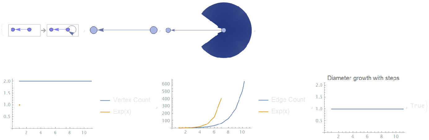
3. "Output Type" -> "Classify" This classifies all the models (including the ones that are filtered out in other output types) into 3 categories : Linear, Exponential, and Neither. It returns an association of these 3 types as Keys and the list of underlying rules and initial state as the values. Here’s an example output:
example3 = WolframModelInterestingRules[{{{1, 2}} {{2, 2}}}, "Output Type" "Classify"]
"Linear"
,"Exponential"
,"Neither"
{{{1,1}}{{1,1},{1,2}},{{1,1}}} |
{{{1,1}}{{1,1},{2,1}},{{1,1}}} |
{{{1,1}}{{2,2},{1,2}},{{1,1}}} |
{{{1,1}}{{2,2},{2,1}},{{1,1}}} |
{{{1,2}}{{1,2},{1,3}},{{1,2}}} |
{{{1,2}}{{1,2},{2,3}},{{1,2}}} |
{{{1,2}}{{2,1},{1,3}},{{1,2}}} |
{{{1,2}}{{2,1},{2,3}},{{1,2}}} |
{{{1,2}}{{1,2},{3,2}},{{1,2}}} |
{{{1,2}}{{2,1},{3,1}},{{1,2}}} |
{{{1,2}}{{1,3},{2,3}},{{1,2}}} |
{{{1,2}}{{1,3},{3,2}},{{1,2}}} |
{{{1,2}}{{2,3},{3,1}},{{1,2}}} |
{{{1,2}}{{1,3},{1,4}},{{1,2}}} |
{{{1,2}}{{3,1},{1,2}},{{1,2}}} |
{{{1,2}}{{3,1},{3,2}},{{1,2}}} |
{{{1,2}}{{3,2},{2,1}},{{1,2}}} |
{{{1,2}}{{3,2},{4,2}},{{1,2}}} |
{{{1,1}}{{1,1},{1,1}},{{1,1}}} |
{{{1,2}}{{1,1},{1,1}},{{1,2}}} |
{{{1,2}}{{1,1},{1,2}},{{1,2}}} |
{{{1,2}}{{1,1},{2,1}},{{1,2}}} |
{{{1,2}}{{1,2},{1,2}},{{1,2}}} |
{{{1,2}}{{1,2},{2,1}},{{1,2}}} |
{{{1,2}}{{2,1},{2,1}},{{1,2}}} |
{{{1,2}}{{2,2},{1,2}},{{1,2}}} |
{{{1,2}}{{2,2},{2,1}},{{1,2}}} |
{{{1,2}}{{2,2},{2,2}},{{1,2}}} |
{{{1,2}}{{1,1},{1,3}},{{1,2}}} |
{{{1,2}}{{2,2},{3,2}},{{1,2}}} |
{{{1,2}}{{1,3},{1,3}},{{1,2}}} |
{{{1,2}}{{3,2},{3,2}},{{1,2}}} |
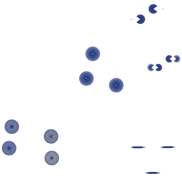
4. “Output Type” -> “FeatureSpacePlot” This outputs a Feature Space Plot of the final states of all the selected models. This is very helpful to just look at everything in one place and identify any models which are different than others. Here is an example of the output:
example4 = WolframModelInterestingRules[{{{1, 2}} {{2, 2}}}, "Output Type" "FeatureSpacePlot"];Rasterize[example4]
Classification of observed growth rates
Classification of observed growth rates
I observed multiple forms of Linear and Exponential growth, but nothing apart from these types of growths. Some of the growths are predictable, others not so much. In general, if the rules or sets of rules which preserve the number of points of application of rules, then the growth rate would be linear. On the other hand, if the number of points of applications of rules increase with each step, then we get an exponential growth. If the number of points of applications of rules decrease with each step, then we get an exponential decay (which I will not discuss here).
Linear
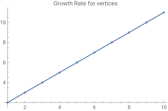
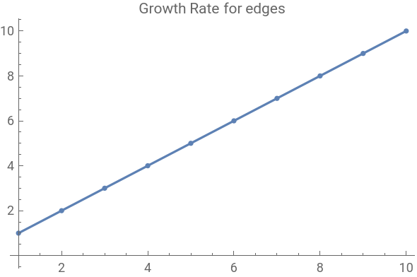
1. Exactly linear growth: This is the growth of the form ‘ax + b’. Consider the following example which preserves the number of points where the rule can be applied. The growth rate for this Wolfram Model is perfectly linear.
rule = {{1, 2}} {{1, 2}, {1, 2, 3}};model = ResourceFunction["WolframModel"][rule, {{1, 2}}, 10, {"VertexCountList", "EdgeCountList"}];modelfit = Table[LinearModelFit[i, x, x], {i, model}];vertexfit = Show[Plot[modelfit[[1]][x], {x, 1, 10}], ListPlot[model[[1]], PlotLabel"Growth Rate for vertices"]]edgefit = Show[Plot[modelfit[[2]][x], {x, 1, 10}], ListPlot[model[[2]], PlotLabel"Growth Rate for edges"]]
2. A small distortion in the beginning and then reaches a linear growth: Here, most of the growth is linear, just the first step shows a small disturbance. For example:
3. Step growth: Here, the overall growth rate is still linear, but it happens in steps. For example, the vertex growth rate for the following model.
Exponential
1. Integer base growth rate: This is an exponential growth where the base of the exponent is an integer. The following example shows a growth rate with the base of 2 for vertices.
2. Non-integer base growth rate: This is an exponential growth where the base of the exponent is not integer. Consider the example below where both the vertices and edges grow exponentially but the base and the constant multiplied by x are not integers.
3. Step growth: Just like the linear step growth, there is also exponential step growth. Here, the overall growth is exponential, but it happens in steps.
Future Work
Future Work
The growth rates for a model depend heavily on the rules and initial condition. So, the future work would include running WolframModelInterestingRules with larger and multiple rules. I have yet to experiment with more than 2 simultaneous rules.
Additionally, the WolframModelInterestingRules does not allow many of the options such as changing the initial condition or the event-ordering in case of multiple rules. Hence, future work will also include upgrading the WolframModelInterestingRules to have some of the options to change the Wolfram Model parameters.
The caveat in all this is the lack of computational power. The number of possible rules increase exponentially when increasing the signature. Hence, a personal computer is unable to run signatures bigger than arity 3.
Another future direction might be to explore the Branchial graphs in the Wolfram Models instead of the Spatial Hypergraphs I explored.
Code Repository
Code Repository
Acknowledgements
Acknowledgements
This project of course could not have been complete without certain people. A huge thanks to Jack Heimrath who went through all the nitty-gritty details with me, Jesse Friedman who helped optimize WolframModelInterestingRules to its best. I would also like to thank Stephen Wolfram, Wolfram Research, and Wolfram Summer School for the opportunity to work on this project.