ORIGINAL ARTICLE: Brian G. Higgins, Housam Binous, A Simple Method for Tracking Turning Points in Parameter Space, JOURNAL OF CHEMICAL ENGINEERING OF JAPAN, 2010, Volume 43, Issue 12, Pages 1035-1042. https://doi.org/10.1252/jcej.10we122.
Article Abstract: We describe a simple method for tracking solutions of nonlinear equations through turning points (also known as limit or saddle-node bifurcation points). Our implementation makes use of symbolic software such as Mathematica to derive an exact system of nonlinear ODE equations to follow the solution path, using a parameterization closely related to arc length. We illustrate our method with examples taken from the engineering literature, including examples that involve nonlinear boundary value problems that have been discretized by finite difference methods. Since the code requirement to implement the method is modest, we believe the method is ideal for demonstrating continuation methods in the classroom.
f(u,α)=0
Using homotopy continuation methods such as the fixed point and the Newton homotopy methods, one can find all real solutions of a polynomial equation .
Solve give the roots of the polynomial equation
In[]:=
(x-0.25)(x-0.75)(x-0.11)(x-2)//Expand
Out[]=
0.04125-0.615625x+2.5175-3.11+
2
x
3
x
4
x
In[]:=
Solve[0.04125`-0.615625`x+2.5175`-3.11`+0,x]
2
x
3
x
4
x
Out[]=
{{x0.11},{x0.25},{x0.75},{x2.}}
Fixed Point Homotopy: H(x,t)=(1-t) (x-x0) + t f(x) with x0=2.5
Fixed Point Homotopy: H(x,t)=(1-t) (x-x0) + t f(x) with x0=2.5
In[]:=
H[x_,t_]:=(1-t)(x-2.5)+t(0.04125`-0.615625`x+2.5175`-3.11`+)
2
x
3
x
4
x
In[]:=
H[x,t]
Out[]=
(1-t)(-2.5+x)+t(0.04125-0.615625x+2.5175-3.11+)
2
x
3
x
4
x
In[]:=
Off[General::"spell"]
In[]:=
MyGrad[fon_,var_List]:=D[fon,#]&/@var
In[]:=
J=MyGrad[H[x,t],{x,t}]
Out[]=
{1-t+t(-0.615625+5.035x-9.33+4),2.54125-1.61563x+2.5175-3.11+}
2
x
3
x
2
x
3
x
4
x
In[]:=
Js=J/.xx[s]/.tt[s]
Out[]=
{1-t[s]+t[s](-0.615625+5.035x[s]-9.33+4),2.54125-1.61563x[s]+2.5175-3.11+}
2
x[s]
3
x[s]
2
x[s]
3
x[s]
4
x[s]
In[]:=
Eq[1]=D[x[s],{s,1}]First[Drop[Js,1]]
Out[]=
′
x
2
x[s]
3
x[s]
4
x[s]
In[]:=
Eq[2]=D[t[s],{s,1}]-First[Drop[Js,{2}]]
Out[]=
′
t
2
x[s]
3
x[s]
In[]:=
sol=NDSolve[{Eq[1],Eq[2],t[0]0,x[0]2.5},{x[s],t[s]},{s,-4.38,0.094},MaxStepFraction0.0005]
Out[]=
x[s]InterpolatingFunction[s],t[s]InterpolatingFunction[s]


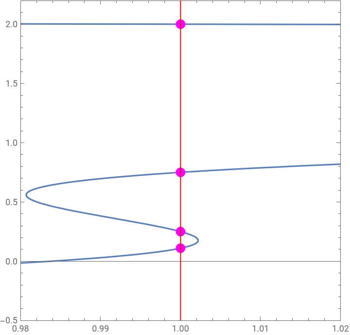
As expected we find four solutions at t=1
In[]:=
plt1=ParametricPlot[{t[s],x[s]}/.sol,{s,-4.3378,0.093},Epilog{RGBColor[1,0,0],Line[{{1,-3},{1,3}}]},PlotRange{{0.98,1.02},{-0.5,2.2}},AspectRatio->1]
Out[]=
In[]:=
l=Graphics[{{RGBColor[1,0,1],PointSize[0.03],Point[{1,0.25}]},{RGBColor[1,0,1],PointSize[0.03],Point[{1,0.75}]},{RGBColor[1,0,1],PointSize[0.03],Point[{1,2}]},{RGBColor[1,0,1],PointSize[0.03],Point[{1,0.11}]}}];
In[]:=
Show[plt1,l,FrameTrue,AspectRatio->1]
Out[]=
In[]:=
sol1=FindRoot[(t[s]/.sol/.sa)1,{a,0.01}]
Out[]=
{a-0.35338}
In[]:=
Evaluate[x[s]/.sol/.sa/.sol1]
Out[]=
{2.}
In[]:=
sol1=FindRoot[(t[s]/.sol/.sa)1,{a,-3}]
Out[]=
{a-3.69175}
In[]:=
Evaluate[x[s]/.sol/.sa/.sol1]
Out[]=
{0.75}
In[]:=
sol1=FindRoot[(t[s]/.sol/.sa)1,{a,-3.8,-4}]
Out[]=
{a-3.94002}
In[]:=
Evaluate[x[s]/.sol/.sa/.sol1]
Out[]=
{0.250001}
In[]:=
sol1=FindRoot[(t[s]/.sol/.sa)1,{a,-4.3,-4}]
Out[]=
{a-4.00048}
In[]:=
Evaluate[x[s]/.sol/.sa/.sol1]
Out[]=
{0.109999}
We have found all solutions on the same single branch because there are no real roots for the equation: f(x) - x + = 0 and x ± ∞. This is a result of our choice of .
x
O
x
O
In[]:=
Solve[0.04125`-0.615625`x+2.5175`-3.11`+-x+2.50,x]
2
x
3
x
4
x
Out[]=
{{x-0.200997-0.880879},{x-0.200997+0.880879},{x1.756-0.171537},{x1.756+0.171537}}
In[]:=
ParametricPlot[{t[s],x[s]}/.sol,{s,-4.337875792747977`,0.09376277513774145`},PlotRange{{-0.05,0.02},{-200,200}},PlotPoints10000,PlotStyleRGBColor[1,0,0],AspectRatio->1]
Out[]=
Newton Homotopy :
H(x,t)= f(x) - (1-t) f(x0) with x0= - 0.5
Newton Homotopy :
H(x,t)= f(x) - (1-t) f(x0) with x0= - 0.5
H(x,t)= f(x) - (1-t) f(x0) with x0= - 0.5
In[]:=
0.04125`-0.615625`x+2.5175`-3.11`+/.x-0.5
2
x
3
x
4
x
Out[]=
1.42969
In[]:=
H[x_,t_]:=-(1-t)(1.4296875)+0.04125`-0.615625`x+2.5175`-3.11`+
2
x
3
x
4
x
In[]:=
J=MyGrad[H[x,t],{x,t}]
Out[]=
{-0.615625+5.035x-9.33+4,1.42969}
2
x
3
x
As expected we find four solutions at t=1
Reference
Reference
M. Kuno and J. D. Seader, Computing All Real Solutions to Systems of Nonlinear Equations with a Global Fixed-Point Homotopy, Ind. Eng. Chem. Res., 1988, 27, 1320-1329.
CITE THIS NOTEBOOK
CITE THIS NOTEBOOK
Homotopy Continuation Method to Find All Root of a Polynomial Equation
by Housam Binous and Ahmed Bellagi
Wolfram Community, STAFF PICKS, April 15 2023
https://community.wolfram.com/groups/-/m/t/2898379
by Housam Binous and Ahmed Bellagi
Wolfram Community, STAFF PICKS, April 15 2023
https://community.wolfram.com/groups/-/m/t/2898379