Standard differential geometry takes place on differentiable manifolds, which have constant, integer dimensions by construction. This is too constricting for the case where you need to deal with a discrete space which can limit to non-integer dimensional space, such as in Wolfram Models. Especial difficulty arises for the tensor formalism of differential geometry, whose indices takes integer values, corresponding to the integer dimensions of the manifold. It is expected that there will be multiple ways to define dot products, which leads to different definitions of orthonormality, which will expectedly have cascading implications for formulating definitions of curvature, tangent spaces and other features from standard differential geometry. This project will construct some definitions of an inner product of vectors in Wolfram Models and explore some of the consequences and features that come from it.
Introduction
Introduction
The concept of vectors is essential for constructing geometric formalisms in any space. Notions from Differential Geometry such as tangent spaces, parallel transport, a connection and more depend on a solid understanding of what vectors are. In a continuous space this is all well established and understood, and even in some discrete settings there have been work on defining and exploring it. The problem, however, comes when working in an arbitrary discrete space, which can also potentially have non-integer dimensions. Considering the scales that most vectors will operate on, and considering that dimension and curvature are statistical features that emerge from larger scale space, care was taken to make no assumption on curvature or dimension. In certain sections where readers might be worried that curvature could interfere, short explanations as to how it is avoided is given where possible. The generality obtained from this approach should also be of great value when studying spaces with fractal, or even varying dimension. The document here is meant as preliminary results, to be taken further in constructing a full theory of geometry on these discrete scales.
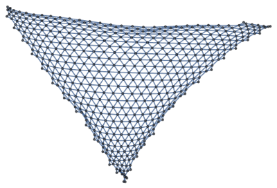
Throughout various graphs will be used to show the ideas laid out. One that will be used extensively comes directly from the Wolfram Model, and is generated by a rule also used by Gorard. It is convenient since it is easy to visualise, and limits to something analogous to flat 2D space. The reader is however encouraged to substitute in graphs of their own to verify that the results obtained are general.
Throughout various graphs will be used to show the ideas laid out. One that will be used extensively comes directly from the Wolfram Model, and is generated by a rule also used by Gorard. It is convenient since it is easy to visualise, and limits to something analogous to flat 2D space. The reader is however encouraged to substitute in graphs of their own to verify that the results obtained are general.
Initializing a graph that will be used repeatedly:
wm=ResourceFunction["WolframModel"];htg=ResourceFunction["HypergraphToGraph"];grph=UndirectedGraph[SimpleGraph[htg[wm[{{x,y,y},{z,x,u}}{{y,v,y},{y,z,v},{u,v,v}},{{1,1,1},{1,1,1}},500]["FinalState"]]]]
Out[]=
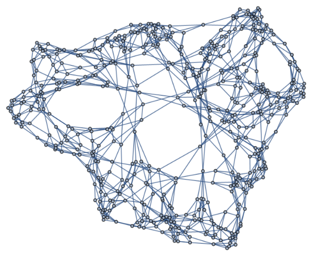
Initializing a graph that limits to a fractal dimension:
frac=UndirectedGraph[SimpleGraph[htg[wm[{{{1,2,3},{1,4,5}}{{2,3,6},{2,3,6},{5,2,6}}},{{1,1,1},{1,1,1}},500]["FinalState"]]]]
Out[]=
Vectors
Vectors
This project will consider three different ways of defining vectors in graphs (and generalizable to hypergraphs and possibly other discrete spaces).
1) Geodesic vectors
1) Geodesic vectors
One way to see vectors is as a geodesic from the origin vertex to a destination vertex, with the length of the vector then also corresponding to the geodesic's length. These vectors are completely described be an ordered set of vertices connected by edges {,,..,}.
v
i
v
2
v
f
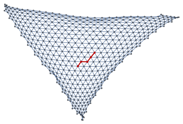
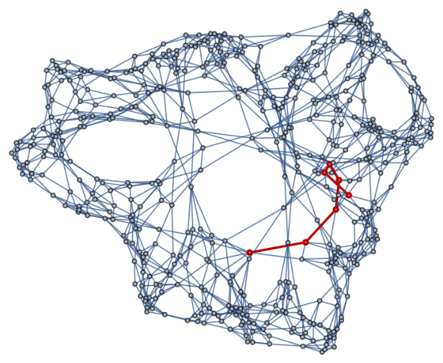
Showing one possible geodesic between two given vertices, unique from other geodesics between the same vertices.
p1=FindShortestPath[grph,143,197];p2=FindShortestPath[frac,59,277];HighlightGraph[grph,Join[Table[p1[[i]]p1[[i+1]],{i,1,Length[p1]-1}],p1],GraphHighlightStyle"Thick"]HighlightGraph[frac,Join[Table[p2[[i]]p2[[i+1]],{i,1,Length[p2]-1}],p2],GraphHighlightStyle"Thick"]
Out[]=
Out[]=
2)Vertex vectors
2)Vertex vectors
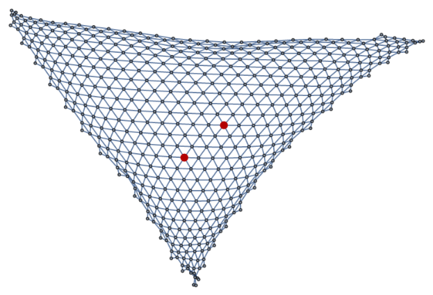
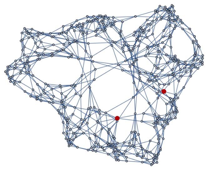
Here we define vectors by only specifying the origin and terminal vertex, with the length of the vector corresponding to the geodesic length between the vertices, but there is no specification of which geodesic corresponds to the vector. These vectors are completely described by an ordered pair of vertices {,}.
v
i
v
f
Showing that only the initial and final vertices matter for this definition.
HighlightGraph[grph,{143,197},VertexSize4]GraphDistance[grph,143,197]HighlightGraph[frac,{59,277},VertexSize4]GraphDistance[frac,59,277]
Out[]=
Out[]=
4
Out[]=
Out[]=
6
3)Abstract length vertex vectors
3)Abstract length vertex vectors
Abstract length vertex vectors are very similar to normal vertex vectors, except we only take the vertex pair to specify something analogous to direction, with the length of the vector needing to be specified separately. These vectors are completely described by an ordered pair of vertices, and a specified length {{,},l}. We can expect some degeneracy, since choosing vertices to indicate direction, is analogous to choosing a point in to specify a unit vector. Showing that multiple vertices in a graph will correspond to the same result of dot products with arbitrary vectors is something that should be possible, but is not attempted here. There is however no obvious reason for this to be true or false in the general case. Therefore no assumptions about the uniqueness of vectors will be made in this analysis. Note also that there is no intrinsic requirement that the abstract length be real, integer or even a number for that matter. Assumptions about the properties of the field over which the length is constructed will be stated where necessary, although these assumptions are only necessary for the given result, not in general. If we were to restrict the abstract length to be equal to the graph distance between the two vertices considered, we can force this construction to be equivalent to the normal vertex vectors. This is therefore a very neat generalisation, that yields some nice extra properties explored below.
v
i
v
f
n
Dot product
Dot product
Here we will explore possible ways of defining the dot product for the given definitions of vectors
1)Geodesic vectors
1)Geodesic vectors
Given the structure we get from defining vectors as geodesics, it allows us a unique construction of the dot product, analogous to dropping a perpendicular from one vector to the other, and then multiplying the length of the projected vector by the length of the vector projected onto to get the dot product. One problem that is immediately apparent, is that there might be multiple legitimate perpendiculars (of equal length) that would lead to different dot products. Here the convention of picking the one with the largest result is chosen.
Represent perpendicular dropped between two vectors, and calculate the dot product between them :
p1=FindShortestPath[grph,143,197];p2=FindShortestPath[grph,143,218];p3=FindShortestPath[grph,197,200];HighlightGraph[grph,{Join[Table[p1[[i]]p1[[i+1]],{i,1,Length[p1]-1}],p1],Style[Join[Table[p2[[i]]p2[[i+1]],{i,1,Length[p2]-1}],p2]],Style[Table[p3[[i]]p3[[i+1]],{i,1,Length[p3]-1}]]},GraphHighlightStyle"Thick"]dt=0;shrt=Infinity;l1=Length[p1]-1;e1=p1[[l1+1]];For[i=Length[p2],i≥1,i--,If[GraphDistance[grph,e1,p2[[i]]]<shrt,shrt=GraphDistance[grph,e1,p2[[i]]];dt=(i-1)*l1;]];Print["The dot product here is:",dt]
There are some obvious issues to this definition. The most severe is that the dot product between vectors with angle more than 90° between them will be 0. There is also the issue that this dot product does not neccesarily commute, and that it sometimes won't give well behaved answers if the perpendicular is dropped from a long vector to one significantly shorter. A possible remedy for both these issues would be to define that the perpendicular is always dropped to the longer vector, although equal lengthed vectors might still not commute. All of this will be covered in the analysis below.
2)Vertex vectors
2)Vertex vectors
Define a function to compute the dot product between two vertex vectors
Represent ' triangle' formed by two vectors, and calculate the dot product between them :
Another possibility arises, in which we can construct something between vertex vectors and geodesic vectors, wherein we identify a vector as the set of all geodesics between two given vertices, where we can take the dot product to be the average of the geodesic dot products between the corresponding sets of geodesics. This can, of course, become extremely computationally expensive for vectors with high geodesic degeneracy, even though they should converge in the limit. It is therefore more of a conceptual tool than a suggestion for a way to practically compute dot products. It also inherits most of the problems of the normal geodesic dot products. We will, however, use this conceptual tool extensively in the section discussing the continuum limits, since it is easy to see how both geodesic- and vertex vectors converge to it. Studying this construction’s characteristic behaviour, therefore, is analogous to studying the behaviour of the other constructions.
Showing the multiple possible geodesics possible between two given vertices
3)Abstract length vertex vectors
3)Abstract length vertex vectors
Define a function to compute the dot product between two abstract length vertex vectors
The reader is encouraged to edit the code above to see for example that the geodesic vector dot product and the abstract vertex vector dot product will not be equal in the general case.
Features of the respective dot products
Features of the respective dot products
1) Geodesic vectors
1) Geodesic vectors
Commutativity
Commutativity
First we can quite easily construct a hypothetical subgraph that shows that the geodesic approach does not commute in general.
Construct a counterexample showing that commutativity is not a general property of geodesic vectors:
Here when the perpendicular is dropped from the red vector onto the yellow vector we get a dot product of 35. If however we consider the perpendicular dropped from the yellow vector onto the red vector, we get a dot product of 16. If we identify the order of multiplication with the direction in which the perpendicular is dropped, this leads to the operation being non-commutative. This also shows a problem where there is a max value of the dot product, which is the square of the length of the vector projected onto. We can make the ad-hoc choice to always project onto the longer vector, which reduces the problem to cases where the vectors are of equal length shown below.
Construct a counterexample showing that commutativity is not a general property of geodesic vectors, even with additional constraints:
Here when the perpendicular is dropped from the red vector onto the yellow vector we get a dot product of 35. If however we consider the perpendicular dropped from the yellow vector onto the red vector, we get a dot product of 28. So there is still ambiguity possible when the vectors are of equal length, which would require more ad-hoc choices to remove.
Scalar multiplication
Scalar multiplication
For geodesics on graphs, scalar multiplication is not unique in general.
Constructing a graph showing how scalar multiplication is not well behaved:
Here we can see that by multiplying the red geodesic by 2, there are multiple possible geodesics of length 4, that overlaps with the original. Therefore vectors as geodesics aren’t well behaved under scalar multiplication in general. We can also see that the dot product won’t be linear under a choice of scalar multiple, illustrated below, with respect to the brown and cyan geodesics.
Constructing an example showing that no result of scalar multiplication gives a satisfactory result in general (with regards to scalar multiplication under a dot product):
Tabulating the result of the dot products between geodesic vectors:
As we can see no geodesic extension will in general be double the dot product with a given geodesic vector, therefore geodesic vector dot products don’t respect scalar multiplication in general under any choice of geodesic extension.
Angles>90°
Angles>90°
It is easy to see that for vectors which are closer to being anti-parallel than parallel, the perpendicular dropped will be along the vector from which it is dropped(which is by definition a geodesic to the origin), such that its projected length will always be 0.
Nonnegative-definite
Nonnegative-definite
Since the dot product is the scalar multiple of 2 graph distances, which is always nonnegative, leading to a nonnegative-definite dot product, not even only in the case of the dot product with itself.
2) Vertex vectors
2) Vertex vectors
Commutativity
Commutativity
Scalar multiplication
Scalar multiplication
The same difficulty of scalar multiplication arises as before, and we can see below that no choice of multiple satisfies what we want in the general case.
Constructing a graph showing how scalar multiplication is not well behaved :
Tabulating the result of the dot products between vertex vectors :
Angles>90°
Angles>90°
We can already see that we get a negative result from the dot product where vectors presumably have more than 90° between them above (for the dot product between green and orange, or between brown and yellow for example).
Nonnegative-definite
Nonnegative-definite
3)Abstract length vertex vectors
3)Abstract length vertex vectors
Commutativity
Commutativity
Scalar multiplication
Scalar multiplication
Angles>90°
Angles>90°
All the results of the normal vertex vector construction applies here.
Nonnegative-definite
Nonnegative-definite
Summary
Summary
Tabulating the results obtained above
General problems with linearity
General problems with linearity
This section is meant to give the reader a brief overview of problems encountered when considering linearity. It is meant to give an idea of why it is not a trivial matter, and requires further work, rather than to give a complete description.
1) Geodesic vectors
1) Geodesic vectors
For geodesic vectors addition quite obviously doesn’t even commute, which immediately casts doubt on its linearity. Even on ‘nice’ graphs where the resultant vector is ‘obvious’ even without a proper definition of parallel transport this problem is easy to show
Initializing a graph that will be used repeatedly for visualisation:
Showing both the initial geodesic vectors and the possible results of their addition:
Here the order in which we stitch the geodesics in clearly matters. We can try and ignore that for a moment and look at how this case would hold up under a dot product
Providing visualisation for the vectors between which a dot product will be taken:
By dropping perpendiculars onto the green vector we can calculate by hand that the dot product with the purple vector+dot product with the orange vector gives 36. The dot product of both resultant vectors with the green vector would be 30. The reader is welcome to calculate that the disparity is even greater if we were to drop the perpendicular from the green vector.
2) Vertex vectors
2) Vertex vectors
While I have already shown some problems that arise during scalar multiplication, I noticeably ignored linearity in its entirety. That is simply because there currently exists no rigorous and general way of adding vectors. This problem arises from lack of a general method of parallel transport. This leads to an ambiguity in the ‘direction’ of the resultant vector. The only constraints we can reasonably put for either vertex or geodesic vectors, is that the resultant vector of a+b must be distance ||a|| from the tip of b, and distance ||b|| from the tip of a. There is also no guarantee that such a vertex even exists. Furthermore there is no reason to expect a single resultant vector to act under the dot product as expected for an arbitrary vector to dot it with.
Visualising vertex vectors that will be considered when attempting to add them:
Showing the overlap in the requirements we can put on final distance of the resultant vector.
We can see that there are three vertices that satisfy the results in this case. We can apply our intuition for how parallel transport should work and claim that the right-most of the three should be the resultant, but this is only possible because we are in a well-behave periodic graph. Constructing a general definition for addition of vertex of geodesic vectors on graphs have proven extremely difficult. Even if we take the ‘obvious result’, we can easily show that it fails under linearity with a dot product under our constructions. Below the orange vertex is the resultant vertex obtained previously from ‘summing’ the yellow and red vertex vectors. We can now show that the sum of the dot products between the red- and purple vectors, and the yellow- and purple vectors, is not the same as the dot product between the resultant orange vector and the purple vector.
It is easy to try it for different examples and show there are many cases where a satisfactory resultant simply doesn’t exist for vertex vectors.
3) Abstract length vertex vectors
3) Abstract length vertex vectors
In the limit
In the limit
There is more than one way of taking a continuum limit of these discrete structures. One way of doing it involves adding vertices in between currently existing ones, and instead of using graph distance, we introduce a notion of a measure, which gives a solid notion of length (from here on referred to as taking an interior limit). The other one involves growing the graph, and considering larger and larger subsets of the graph (from here on referred to as taking the exterior limit). Here I discuss how I expect the vectors and dot products to act in the limit, with reasoning, but not a graph theoretic/empirical proof. Doing that is a potential for further work. The intrinsic and extrinsic limits respectively are visualised below.
1) Geodesic vectors
1) Geodesic vectors
2) Vertex vectors
2) Vertex vectors
3) Abstract length vertex vectors
3) Abstract length vertex vectors
Normal vertex vectors are expected to be able to represent any real valued length in the limit, making them identical to abstract length vertex vectors constructed with real numbers. There is of course the possibility of using something other than reals for the length, which will not necessarily be reconstructable even in the limit of vertex vectors. There is no reason to expect that abstract length vertex vectors will act significantly differently to vertex vectors (ignoring some of the freedoms of abstract length).
Conclusion
Conclusion
Three ways of defining vectors in discrete spaces were identified, with corresponding definitions for weakened dot products(linearity not necessarily satisfied). The consequences and properties of these definitions were properly explored and proved where possible, and some expectations for the limiting cases were put forward (with some limited empirical evidence to back it up). Although all three definitions are expected to correspond to conventional vectors in a large enough limit, some differences in their discrete behaviours was obvious. The notion of an abstract length vertex vector seems to be the most promising in its discrete behaviour and properties, although great care will necessarily need to be taken in order to define addition. Placing certain constraints on the possible values of the abstract length also seems like a promising possibility. Some of the problems that arise when considering linearity was explored, and should prove important in any attempt to define vector addition and everything that comes with it.
Further Work
Further Work
The reader will have encountered several possibilities for further work raised in the document. A lot of potential lies in doing more empirical work to solidify assertions made that are not necessarily possible to rigorously show mathematically. More work on understanding and solidifying the limiting behaviour of the structures defined above is also a necessary avenue to explore. A natural continuation of the bulk of the work done above (briefly alluded to in the section on linearity) is exploring definitions of parallel transport, affine connections, vector addition and tangent spaces. These are essential next steps on the way to fully understanding discrete non-integer dimensional geometry. Extending the work done here to the language of differential forms, as well as other exterior calculus concepts seems like an exciting prospect. The lynchpin there will expectedly be defining a rigorous wedge product, as well as establishing a notion of a tangent space. The author urges anyone continuing any of the work done here to establish as much as possible without referring to dimension and/or curvature. Reasons are stated in the introduction. This seems to be a very fruitful direction, with a lot of potential work that can be done to extend this project.
Keywords
Keywords
◼
Vector
◼
Graph
◼
Dot product
◼
Fractional Dimensions
◼
Discrete Geometry
◼
Discrete Vectors
Acknowledgment
Acknowledgment
Mentor: Cameron Beetar
Special thanks to Cameron Beetar, Jonathan Gorard and Xerxes Arsiwalla for the extended conversations which helped me formalise my sometimes crazy( or as Cameron would put it, cheeky) ideas. The idea of a geodesic vector and its dot product comes from Jonathan, and the idea for vectors as the set of all geodesics between to vertices and its corresponding dot product comes from Cameron.
In my quest to understand the Wolfram Models, the documents written by Stephen Wolfram and Jonathan as well as the code written by Max Piskunov were indispensable sources of information, explanation and direction.
I also appreciate the in depth answers provided by Erin Cherry, José Caballero, Tobias Canavesi, Hatem Elshatlawy, Nikolay Murzin, Max, Jonathan, Cameron and Xerxes for my wide range of questions.
Thank you to Simeon Boshoff who helped create visualisations of the two types of limits.
Finally, I also wish to express my gratitude towards the entire winter school and everyone who participated for making this truly enlightening and stimulating experience possible. Everyone I interacted with was open minded, helpful and incredibly friendly, which enriched the entire experience.
References
References
◼
Gorard, J., 2020. Some Relativistic and Gravitational Properties of the Wolfram Model. arXiv preprint arXiv:2004.14810.