This lecture series on stochastic processes in Wolfram Language is now available on YouTube.
Below is an example lecture: Geometric Brownian Motion
Below is an example lecture: Geometric Brownian Motion
Contents
Contents
◼
Basic properties of GBM processes
◼
Examples of GBM processes
◼
State properties for a GBM process
◼
PDF and event probabilities
◼
Autocorrelation, stationarity and independence
◼
Applications
◼
Modeling stocks and indices
◼
Derivatives pricing and sensitivities
Geometric Brownian Motion
Geometric Brownian Motion
◼
GeometricBrownianMotionProcess[μ,σ,]
x
0
x
0
◼
Widely used for modeling stock price processes
◼
A continuous time, continuous state model
◼
The state satisfies an Ito differential equation: x (t) = μ x(t)t + σ x(t) w (t)where w is a standard Wiener process
◼
The state x(t) follows a )t + Log[], and standard deviation
LogNormalDistributionwithmeanμ-
2
σ
2
x
0
σ
t
Example
Example
In[]:=
data=RandomFunction[GeometricBrownianMotionProcess[.1,0.5,100],{0,1,.01},4]
In[]:=
ListLinePlot[data,FillingAxis,ImageSizeLarge]
Compare Paths for Different Drift Parameter Values
Compare Paths for Different Drift Parameter Values
Compare Paths with Different Volatilities
Compare Paths with Different Volatilities
State Properties
State Properties
Distribution of the Continuous State
Distribution of the Continuous State
The state of a GBM process at time t follows a LogNormal Distribution
In[]:=
xGeometricBrownianMotionProcess[μ,σ,][t]
x
0
Out[]=
xLogNormalDistributiontμ-+Log[],
2
σ
2
x
0
t
σLet' s take a look at some examples of the LogNormally distributed price process x(t) at various times t, for a specific set of GBM parameters:
In[]:=
Plot[Evaluate@Table[PDF[GeometricBrownianMotionProcess[0,1,1][t],x],{t,{1/2,1,2}}],{x,0,3},FillingAxis,PlotLegends{"t = 1/2","t = 1","t = 2"},ImageSizeLarge]
Mean
Mean
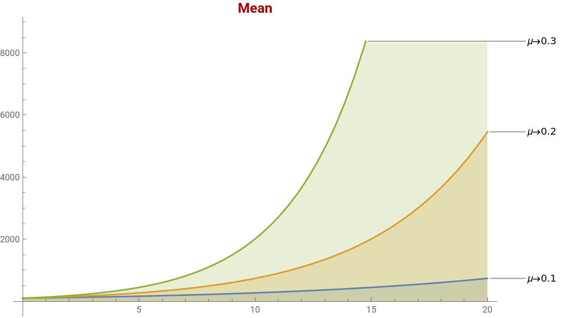
The state mean grows exponentially over time, with growth rate governed by the process drift:
In[]:=
Mean[GeometricBrownianMotionProcess[μ,σ,][t]]//Simplify
x
0
Out[]=
tμ
x
0
In[]:=
StateMean[t_]:=Mean[GeometricBrownianMotionProcess[μ,σ,][t]]/.100//Simplify
x
0
x
0
In[]:=
Plot[{StateMean[t]/.μ0.1,StateMean[t]/.μ0.2,StateMean[t]/.μ0.3},{t,0,20},PlotLabel->Style["Mean",Darker[Red],Bold,14],PlotLabels->{"μ→0.1","μ→0.2","μ→0.3"},FillingAxis,ImageSizeLarge]
Out[]=
Standard Deviation
Standard Deviation
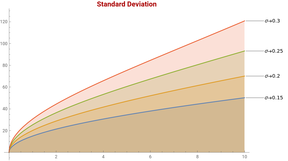
The state standard deviation is a function of the initial value, time, drift and process volatility:
In[]:=
StandardDeviation[GeometricBrownianMotionProcess[μ,σ,][t]]//Simplify
x
0
Out[]=
2tμ
t
2
σ
2
x
0
In[]:=
StDev[t_]:=StandardDeviation[GeometricBrownianMotionProcess[μ,σ,][t]]/.{μ0}/.100//Simplify
x
0
x
0
In[]:=
Plot[{StDev[t]/.σ0.15,StDev[t]/.σ0.20,StDev[t]/.σ0.25,StDev[t]/.σ0.30},{t,0,10},PlotLabels->{"σ→0.15","σ→0.2","σ→0.25","σ→0.3"},PlotLabel->Style["Standard Deviation",Darker[Red],Bold,14],FillingAxis,ImageSizeLarge]
Out[]=
Skewness
Skewness
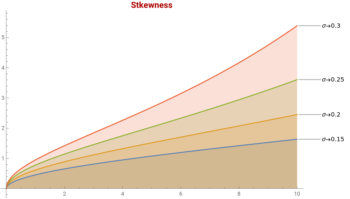
State skewness grows exponentially over time with growth rate governed by the process variance:
In[]:=
Skewness[GeometricBrownianMotionProcess[μ,σ,Subscript[x,0]][t]]//Simplify
Out[]=
-1+
2+t
2
σ
t
2
σ
In[]:=
skew[t_]:=Skewness[GeometricBrownianMotionProcess[μ,σ,][t]]//Simplify
x
0
Plot[{skew[t]/.σ0.15,skew[t]/.σ0.20,skew[t]/.σ0.25,skew[t]/.σ0.30},{t,0,10},PlotLabel->Style["Skewness",Darker[Red],Bold,14],PlotLabels->{"σ→0.15","σ→0.2","σ→0.25","σ→0.3"},FillingAxis,ImageSizeLarge]
Out[]=
Kurtosis
Kurtosis
State kurtosis grows exponentially over time with growth rate governed by the process variance :
In[]:=
Kurtosis[GeometricBrownianMotionProcess[μ,σ,][t]]
x
0
Out[]=
-3+3+2+
2t
2
σ
3t
2
σ
4t
2
σ
In[]:=
kurt[t_]:=Kurtosis[GeometricBrownianMotionProcess[μ,σ,][t]]
x
0
In[]:=
Plot[{kurt[t]/.σ0.15,kurt[t]/.σ0.20,kurt[t]/.σ0.25,kurt[t]/.σ0.30},{t,0,10},PlotLabel->Style["Kutosis",Darker[Red],Bold,14],PlotLabels->{"σ→0.15","σ→0.2","σ→0.25","σ→0.3"},FillingAxis,ImageSizeLarge]
State PDF and Probabilities
State PDF and Probabilities
PDF
PDF
We can calculate the PDF directly from the underlying process:
Expectation of an Expression
Expectation of an Expression
Probability of an Event
Probability of an Event
Autocorrelation, Stationarity
Autocorrelation, Stationarity
Modeling a Stock index
Modeling a Stock index
Download daily data for the S&P 500 Index
Download daily data for the S&P 500 Index
Estimate a GBM process representing the index:
Estimate a GBM process representing the index:
Simulate future paths for the next 100 days
Simulate future paths for the next 100 days
Calculate the mean of the simulated paths to find predicted values:
Plot the sample paths and process mean
Plot the sample paths and process mean
Modeling Stock Returns
Modeling Stock Returns
Mean
Mean
Variance
Variance
Distribution of stock returns in GBM process
Distribution of stock returns in GBM process
Returns as a Wiener process
Returns as a Wiener process
Option Pricing and Sensitivity
Option Pricing and Sensitivity
Call Option Payoff
Call Option Payoff
Next we look at how to derive the pricing formula and Greeks for simple option products.
A call option with strike price k gives the holder of the option to purchase a stock at price k. He will do this providing the stock price at time t, x[t] > k.
The payoff from a European call option at expiration is the expected value of Max[x(t)-K, 0], where K is the strike price.
The payoff from a European call option at expiration is the expected value of Max[x(t)-K, 0], where K is the strike price.
Option Expectation
Option Expectation
We can evaluate this expectation directly for a general GBM process :
Next, we will price a specific call option and check that the pricing formula we derived matches the result given by the Wolfram Language FinancialDerivative function:
Option Value vs Volatility
Option Value vs Volatility
Let’s take a look at how a call option value varies over time, with different levels of annual volatility in the range 10% to 50%.
Option Sensitivities (“Greeks”)
Option Sensitivities (“Greeks”)
In order to derive the formulae for the option sensitivities (“Greeks”), we take the derivative of the option pricing formula with respect to each parameter.
Delta
Delta
Let’s check the delta for a specific option, using this derived formula:
Theta
Theta
We can do the same for theta, which measures the rate of decay in the option value :
The values of delta and theta calculated from the above derivations are very close to the theoretical values:
Summary
Summary
◼
We showed how to derive option pricing formula directly from the pdf of stock price, the state variable x(t)in a Geometric Brownian Motion Process
◼
Likewise, we demonstrated how to calculate the option Greeks, by taking the derivative of the option value w.r.t. the option parameters x, t and σ
Geometric Brownian Motion 3D
Option Greeks
Option Greeks
Call Option Greeks
Call Option Greeks
CITE THIS NOTEBOOK
CITE THIS NOTEBOOK
Lecture series on Stochastic Processes
by Jonathan Kinlay
Wolfram Community, STAFF PICKS, January 12, 2023
https://community.wolfram.com/groups/-/m/t/2777429
by Jonathan Kinlay
Wolfram Community, STAFF PICKS, January 12, 2023
https://community.wolfram.com/groups/-/m/t/2777429