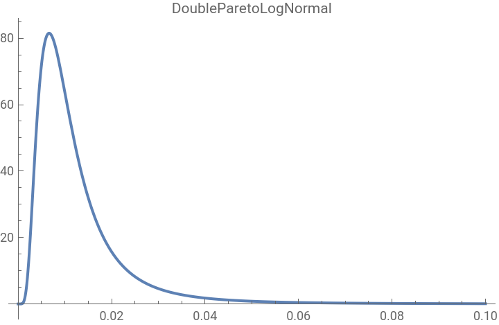
DoubleParetoLogNormal Distribution is now a ResourceFunction
DoubleParetoLogNormal Distribution is now a ResourceFunction
The NormalLaplaceDistribution is also available as a resource function. The functions were revised so that they work independently of each other.
In[]:=
DPLN=ResourceFunction["DoubleParetoLogNormalDistribution"]
Out[]=
In[]:=
NL=ResourceFunction["NormalLaplaceDistribution"]
Out[]=
Here is an example of using the DoubleParetoLogNormalDistribution to give a better tail fit to data of a volatility measure than does the generalized extreme value distribution. See A simple intraday volatility measure. Quiet is used because the range of values gets outside machine numbers for a compiled function which reverts to non-compiled version.
In[]:=
ts=FinancialData["SPY","OHLC",{2008}];lnhilo=Log[#2/#3]&@@@Normal[QuantityMagnitude[ts]["Values"]];dplnD=Quiet@EstimatedDistributionlnhilo,[α,β,μ,σ]
Out[]=
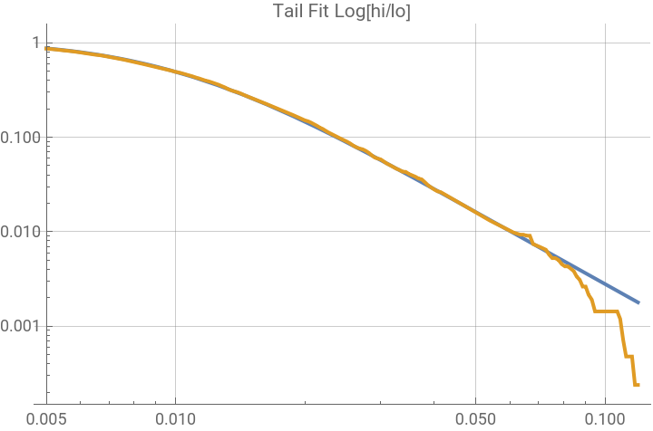
The tail fit misses only the last three points of the data, which are not likely accurately represented in the EmpiricalDistribution, given the size of the sample. On the LogLog plot the right tail plotted as a survival function becomes linear.
In[]:=
empD=EmpiricalDistribution[lnhilo];LogLogPlot[{1-CDF[dplnD,x],1-CDF[empD,x]},{x,0.005,Max[Abs[lnhilo]]},GridLines->Automatic,PerformanceGoal->"Speed",PlotLabel->"Tail Fit Log[hi/lo]"]

-152
10
-234
10
Out[]=
Goodness of fit testing.
In[]:=
HT=DistributionFitTest[lnhilo,dplnD,"HypothesisTestData"];HT["TestDataTable",All]
Out[]=
Statistic | P-Value | |
Anderson-Darling | 0.641106 | 0.60999 |
Cramér-von Mises | 0.0975762 | 0.596888 |
Kolmogorov-Smirnov | 0.0111657 | 0.668791 |
Kuiper | 0.0199965 | 0.375115 |
Pearson 2 χ | 68.9203 | 0.115111 |
Watson 2 U | 0.0959481 | 0.299845 |
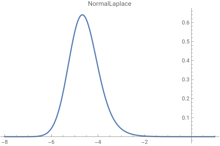
The log of the data has the shape of a NormalLaplaceDistribution; the fitting is easier using the Log[data], so it is the NormalLaplaceDistribution which is used for fitting. Both ResourceFunctions are written so that they are independent, but they use the same code.
In[]:=
nlfit=Quiet@EstimatedDistribution[Log[lnhilo],NL[α,β,μ,σ]]dplnD
Out[]=
Out[]=
The functions are designed so the parameters look the same but the functions are very different, similar to the Normal and LogNormal distributions.
In[]:=
Plot[PDF[nlfit,x],{x,-8,1},PlotRange->All,PlotLabel->"NormalLaplace"]Plot[PDF[dplnD,x],{x,0,0.1},PlotRange->All,PlotLabel->"DoubleParetoLogNormal"]
Out[]=
65.6841
2.04286×
-6
10
Out[]=