ArpaAlohaEtherInternet: distributed algorithms for broadcast queues
Backoff Story of 1/Q
by Bob Metcalfe
Backoff Story of 1/Q
by Bob Metcalfe
You may be starting a new career; this is the start of my sixth.
I am a fledgling "computational engineer" after decade-long careers in engineering, entrepreneurship, journalism, venture capital, and the startup ecosystem of Austin, Texas. To get started, I just joined MIT's Computer Science and Artificial Intelligence Lab (CSAIL) as a Research Affiliate.
I have spent the first three weeks of my new career at Wolfram Summer School 2022.
Having been an Internet pioneer since 1970, I am sharing here ideas about the Arpanet, Alohanet, Ethernet, and Internet, hence ArpaAlohaEtherInternet.
Now
Out[]=
This notebook goes back to 1970 and the Alohanet at The University of Hawaii. There, Professor Norm Abramson RIP studied multi-access radio channels, shared using randomized retransmissions. I spent a month in Hawaii with Abramson figuring out to incorporate randomized retransmissions into Ethernet. (Have I mentioned that I invented Ethernet on May 22, 1973 -- 49 years ago?) Abramson modeled the efficiency of Alohanet. I’ve recreated Norm's model here in Wolfram Language.
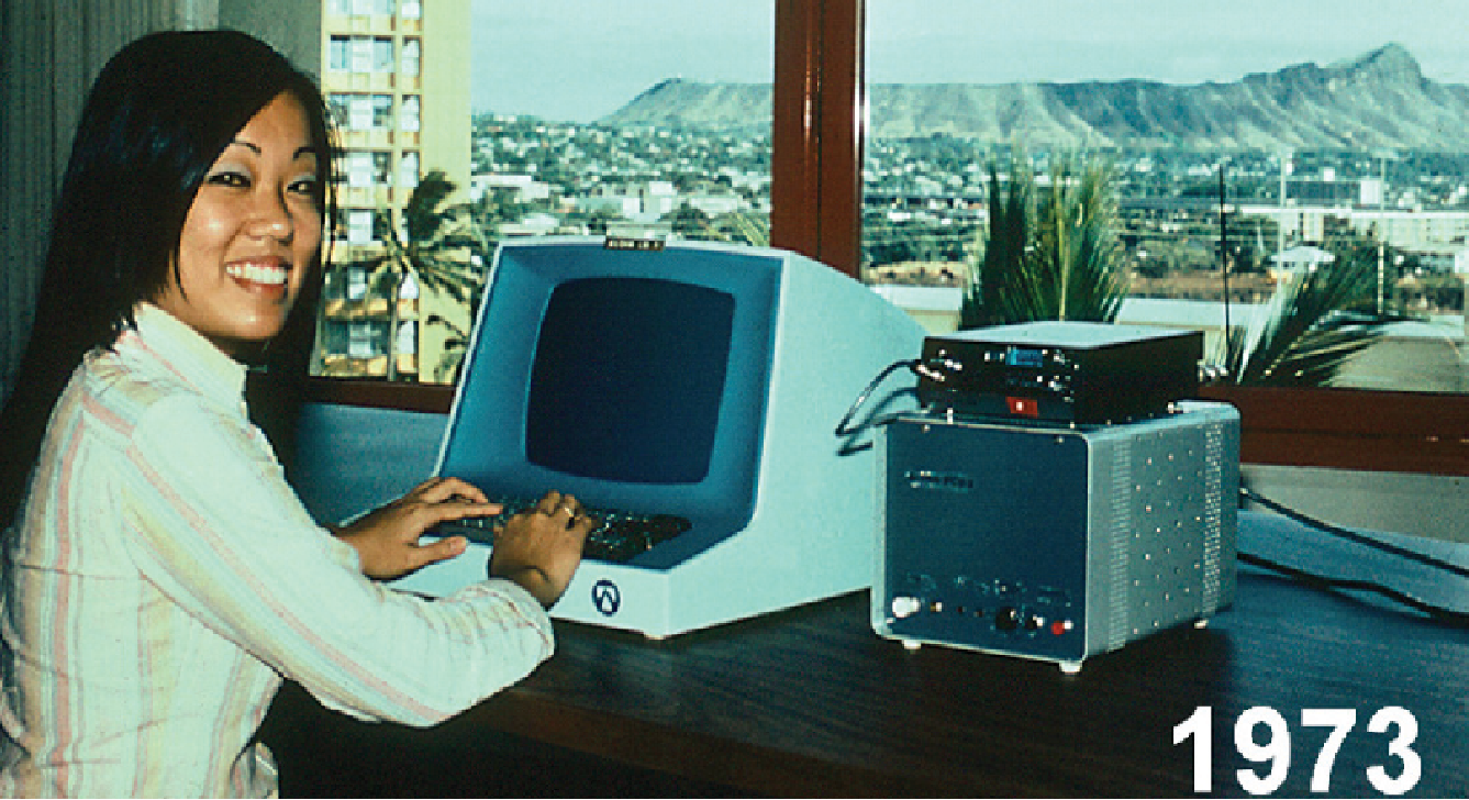
Alohanet
Alohanet
Ethernet
Ethernet
Ethernet Communications of the ACM Model (1976) by Bob Metcalfe
ACM = Association for Computing Machinery
ACM = Association for Computing Machinery
Calculating CSMA/CD Ethernet efficiencies over loads and packet lengths.
The key improvement of Ethernet over Alohanet is carrier sense, with which short Ethernet contention intervals are amortised over long transmission intervals.
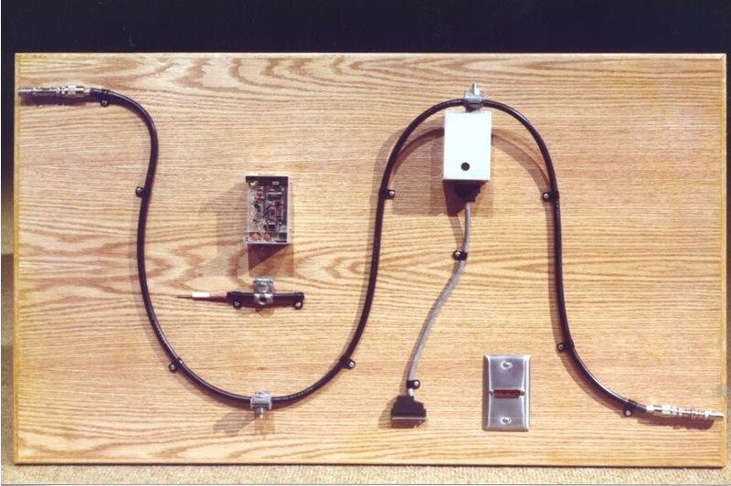
Ethernet paper variable names are preserved with an e at the front of each.
eP is bits per packet, today maximum is 1,518 bytes or 12,144 bits
In[]:=
eP=4096;
eC is capacity of channel in bits per second
first Ethernet 2.94Mbps, today 10/100Mbps, 1/10/100//800 Gbps
first Ethernet 2.94Mbps, today 10/100Mbps, 1/10/100//800 Gbps
In[]:=
eC=3000000;
eT is slot time in seconds
In[]:=
eT=0.000016;
eQ is number of stations queued
A = Probability (prob) of 1 station transmitting, q stations each with probability x; x max?
In[]:=
ClearAll[eA]eA[x_,q_]:=q*x(1-x)^(q-1)
There is a probability p of transmission that maximizes A, for example for q==10
Again, eA is the probability of 1 out of q stations transmitting
x used for probability of xmit
Again, eA is the probability of 1 out of q stations transmitting
x used for probability of xmit
In[]:=
Plot[eA[x,10],{x,0.,1.},AxesLabel->{"x","Probability"}]
Out[]=
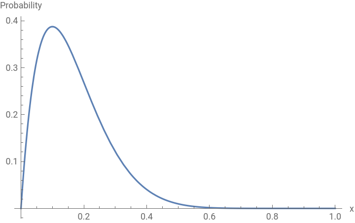
Find p that maximizes 1 xmitter among q stations
Take the derivative, set equal to 0, solve:
p is 1 for q ==1, but what about for q>1?
Major finding: optimal backoff is 1/q
Take the derivative, set equal to 0, solve:
p is 1 for q ==1, but what about for q>1?
Major finding: optimal backoff is 1/q
In[]:=
Solve[D[eA[x,q],x] == 0&&(q>1)&&(0<x<1),x]
Out[]=
x
x xmit prob that maximizes prob of just 1 among q is 1/q. True for q=1 also. Backoff result.
In[]:=
maxprob=ReplaceAll[eA[x,q],x->(1/q)]
Out[]=
-1+q
1-
1
q
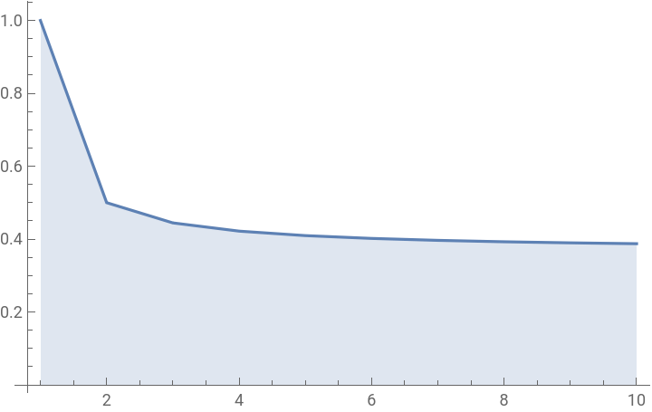
Now, the max prob of uncollided xmission of q stations
In[]:=
eAm[q_] := If[q<2, 1.0, maxprob]
q=1 is a special case, eAm[1] == 1.0, but formula gets 0^0, not defined, so fix with q<2
In[]:=
ClearAll[maxxmitprobs]maxxmitprobs = Table[eAm[q],{q,1,10}]//N;
Maximum transmit probability as a function of q, queued stations
In[]:=
ListLinePlot[maxxmitprobs, Filling->Axis, PlotRange->All]
Out[]=
Mean waiting time
In[]:=
ClearAll[eW]eW[ewA_] := If[0.0<ewA<1.0, (1.0-ewA)/ewA, 0.0]
In[]:=
ListLinePlot[Table[eW[a],{a,.01,1.,.1}],Filling->Axis,PlotRange->All]
Out[]=
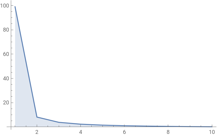
Ethernet Channel Efficiency (eE)
Ethernet Channel Efficiency (eE)
eeP = packet length, eeQ is number of stations, eC is capacity
eW = mean waiting time
eA = prob of 1 xmit given q
eT = turnaround time
x = prob of xmit by q stations
eW = mean waiting time
eA = prob of 1 xmit given q
eT = turnaround time
x = prob of xmit by q stations
Efficiency is time good divided by time good plus contention.
A for probability of acquisition
W is mean number of slots waiting for acquisition
E is for efficiency
Table of Ethernet efficiencies per packet sizes and number of contenders
This table is an exact copy of the Ethernet efficiency table in 1976 CACM paper.
You will notice that efficiencies of Ethernet are greater than Alohanet’s 18%.
You will notice that efficiencies of Ethernet are greater than Alohanet’s 18%.
Distributed Algorithms for Broadcast Queues
Distributed Algorithms for Broadcast Queues
Here we set the width and length of the next simulation
This model is based on a table (list) of station associations, each association containing a station’s ID, state, counter “mean,” and delay (count down state). Here is a list of the states. They are processed by the model’s state machine, below.
Iterate state machine on stations