ABSTRACT(original article): The laminar flow reactor (LFR) is one of the most comprehensive problems in chemical reaction engineering, as its modeling involves mass, heat, and momentum conservation equations coupled with chemical reaction rate equations. It is relatively easy to grasp its basic operation, but the solution of the problem is far from trivial. Although there are analytical solutions that simplify the problem, students and tutors must use efficient numerical strategies to appropriately solve some LFR problems. In the present investigation, we solve several different cases of two-dimensional cylindrical LFR, beginning with the isothermal case as a benchmark. Calculations were performed using the Chebyshev orthogonal collocation technique by custom scripts in Scilab, Mathematica©, and Matlab®, and were compared with solutions available from the ECRE version of COMSOL®, which was used as the reference, as well as available analytical solutions in the literature. After analyzing the case of the isothermal LFR with Newtonian fluid, we explored non-Newtonian fluids, including Carreau and Bingham fluids, whose LFR results are not available in the preceding literature. For Newtonian fluids, besides (a) the isothermal case, we also explore three other non-isothermal design cases: (b) cooling jacket with a fixed heat exchange coefficient at the wall, (c) adiabatic operation, (d) non-isothermal LFR with isothermal wall. Through a performance criterion, the different operation models are compared and we show that non-isothermal design cases perform better than the isothermal case. Computation times for different scenarios are quite short, and taking 25 nodal points or more suffices for an accurate and timely solution of the more complex problem, Case (b). The numerical modeling approach is useful from a pedagogical standpoint, as one can compare numerical results with classical assumptions, and progress from a more restrictive conceptual model (segregated flow) to an array of different kinds of operation with the LFR, in which one needs to consider diffusion and temperature distribution. CITATION (original article): A.-H. Soares, L. de Sousa Santos, H. Binous, A. A. Shaikh, and A. Bellagi, Exploring tubular steady-state laminar flow reactors with orthogonal collocation, Comput. Appl. Eng. Educ. (2024), e22795. DOI: https://doi.org/10.1002/cae.22795
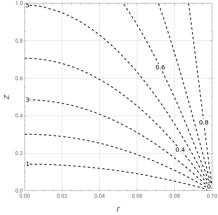
This problem was first proposed by Professor Fogler of Univ. of Michigan, Ann-Arbor, using COMSOL - ECRE (see Ref. 1). Here, we reproduce Figure 9 of Ref . 2, which gives the contour plot of the conversion in an adiabatic laminar flow reactor (Newtonian fluid case).
We also draw the density plot. Finally, the value of the mixing cup concentration is computed. Our solution is based on the Chebyshev Orthogonal Collocation Technique.
We also draw the density plot. Finally, the value of the mixing cup concentration is computed. Our solution is based on the Chebyshev Orthogonal Collocation Technique.
number of collocation points is Np+1
Np=30;
Differentiation matrix
Ds=Table[d[i,j],{i,0,Np},{j,0,Np}];d[0,0]=(2Np^2+1)/6//N;d[Np,Np]=-(2Np^2+1)/6//N;d[i_,i_]:=-y[i]/(2(1-y[i]^2));y[i_]:=Cos[iPi/Np]//N;d[j_,k_]:=If[j≠k,c[j](-1)^(j+k)/(c[k](y[j]-y[k]))];c[i_]:=If[i0||iNp,2,1];Dsq=Ds.Ds;
Reactor dimensions
R=0.1;L=1;
Partial derivative operators
L2r=(2/R)^2KroneckerProduct[Dsq,IdentityMatrix[Np+1]];L2z=(2/L)^2KroneckerProduct[IdentityMatrix[Np+1],Dsq];L1r=(2/R)KroneckerProduct[Ds,IdentityMatrix[Np+1]];L1z=(2/L)KroneckerProduct[IdentityMatrix[Np+1],Ds];
Concentrations, conversions, temperatures
Ca=Table[ca[i+(j-1)(Np+1)],{j,1,Np+1},{i,1,Np+1}]//Flatten;xa=Table[1-ca[i+(j-1)(Np+1)]/Ca0,{j,1,Np+1},{i,1,Np+1}]//Flatten;T=Table[t[i+(j-1)(Np+1)],{j,1,Np+1},{i,1,Np+1}]//Flatten;Ta=Table[ta[j],{j,1,Np+1}]//Flatten;(*walltemperaturesarelabeledTa*)
Derivatives of wall temperatures
Tap[i_]:=(2/L)(Ds[[i,j]]Ta[[j]])
Np+1
∑
j=1
Collocation point positions
Radial positions
In[]:=
r=Table[R/2(1+y[i]),{i,Np,0,-1}]
Out[]=
{0.,0.000273905,0.00109262,0.00244717,0.00432273,0.00669873,0.00954915,0.0128428,0.0165435,0.0206107,0.025,0.0296632,0.0345492,0.0396044,0.0447736,0.05,0.0552264,0.0603956,0.0654508,0.0703368,0.075,0.0793893,0.0834565,0.0871572,0.0904508,0.0933013,0.0956773,0.0975528,0.0989074,0.0997261,0.1}
Axial positions
In[]:=
z=Table[L/2(1+y[i]),{i,Np,0,-1}]
Out[]=
{0.,0.00273905,0.0109262,0.0244717,0.0432273,0.0669873,0.0954915,0.128428,0.165435,0.206107,0.25,0.296632,0.345492,0.396044,0.447736,0.5,0.552264,0.603956,0.654508,0.703368,0.75,0.793893,0.834565,0.871572,0.904508,0.933013,0.956773,0.975528,0.989074,0.997261,1.}
Governing equations:
Mass balance
Eq1[i_]:=-Dp1/r[[Quotient[i-1,Np+1]+1]]L1r[[i]].Ca+DpL2r[[i]].Ca+DpL2z[[i]].Ca+2U(1-(r[[Quotient[i-1,Np+1]+1]]/R)^2)L1z[[i]].Ca+ra[i]0;
Energy balance
Eq2[i_]:=-k1/r[[Quotient[i-1,Np+1]+1]]L1r[[i]].T+kL2r[[i]].T+kL2z[[i]].T+2U(1-(r[[Quotient[i-1,Np+1]+1]]/R)^2)rhoCpL1z[[i]].T+DHra[i]0;
Adiabatic reactor case. Hence the derivatives at the wall are zero. To do so, we set Uk=0
Eq3[i_]:=Tap[i]-2PiRUk/(mcCpc)(T[[i+(Np)(Np+1)]]-Ta[[i]])
Values of the parameters obtained from COMSOL-ECRE see Ref. 1
Uk=0;Cpc=4180;mc=0.01;k=0.559;DH=-83680;Dp=10^-9;Ea=95238;A=1.110^8;rho=1000;Cp=4180;U=v0/(PiR^2);Rg=8.314;v0=510^-4;Ta0=298;Keq0=1000;rhocat=1500;T0=320;Ca0=500;
Rate equation - reversible second-order
ra[i_]:=-AExp[-Ea/(RgT[[i]])]rhocat(Ca[[i]]^2-1/(Keq0Exp[DH/Rg(1/303-1/T[[i]])])(2Ca0xa[[i]])^2)
Boundary conditions
BC1=Table[Ca[[1+(j-1)(Np+1)]]==Ca0,{j,1,Np+1}];BC2=Table[L1r[[i+Np(Np+1)]].Ca==0,{i,2,Np}];BC3=Table[L1r[[i]].Ca==0,{i,2,Np}];BC4=Table[L1z[[Np+1+(j-1)(Np+1)]].Ca==0,{j,1,Np+1}];BC5=Table[T[[1+(j-1)(Np+1)]]T0,{j,1,Np+1}];BC6=Table[L1r[[i]].T==0,{i,2,Np}];BC7=Table[L1z[[Np+1+(j-1)(Np+1)]].T==0,{j,1,Np+1}];BC8=Table[L1r[[i+Np(Np+1)]].TUk/k(T[[i+Np(Np+1)]]-Ta[[i]]),{i,2,Np}];BC9=Ta[[1]]Ta0;
Unknown concentrations
In[]:=
unknowns=Join[Flatten[Table[{{Ca[[i]],300},{T[[i]],340}},{i,1,(Np+1)(Np+1)}],1],Table[{Ta[[i]],320},{i,1,Np+1}]];
System of equations to be solved using FindRoot
In[]:=
sys=Flatten[Join[{BC1,BC2,BC3,BC4,BC5,BC6,BC7,BC8,BC9,Flatten[Table[{Eq1[i+(j-1)(Np+1)],Eq2[i+(j-1)(Np+1)]},{i,2,Np},{j,2,Np}]],Table[Eq3[i],{i,2,Np+1}]}],1];
Check : the number of equations matches the number of unknowns
In[]:=
Length[unknowns]
Out[]=
1953
In[]:=
Length[sys]
Out[]=
1953
In[]:=
sol=Quiet@FindRoot[sys,unknowns];
Contour Plot of the Conversion
Contour Plot of the Conversion
In[]:=
a=Flatten[Table[{r[[j]],z[[i]],1-Ca[[i+(j-1)(Np+1)]]/Ca0/.sol},{j,1,Np+1},{i,1,Np+1}],1];f=Interpolation[a,InterpolationOrder3]
Out[]=
InterpolatingFunction


A few selected contours between 0 and 1
ctrs=Table[i,{i,0.1,0.9,0.1}]
Out[]=
{0.1,0.2,0.3,0.4,0.5,0.6,0.7,0.8,0.9}
In[]:=
p2=ContourPlot[f[x1,y1],{x1,0,0.1},{y1,0,1},Contoursctrs,PlotPoints100,FrameLabel{Style["r",Italic,16],Style["z",Italic,16]},PlotLegendsAutomatic,ContourStyleTable[{Black,Dashed,Thickness[0.004]},{i,1,8}],ContourShadingNone,GridLines->Automatic,AxesOrigin{0,0},ContourLabels->(Text[#3,{#1,#2},BackgroundWhite]&),PlotRange->{{0,0.1},{0,1}}]
Out[]=
In[]:=
p2b=ContourPlot[f[x1,y1],{x1,0,0.1},{y1,0,1},Contoursctrs,PlotPoints100,FrameLabel{Style["r",Italic,16],Style["z",Italic,16]},PlotLegendsAutomatic,ContourStyleTable[{Black,Dashed,Thickness[0.004]},{i,1,8}],ColorFunction"Rainbow",GridLines->Automatic,AxesOrigin{0,0},ContourLabels->(Text[#3,{#1,#2},BackgroundWhite]&),PlotRange->{{0,0.1},{0,1}}]
Out[]=
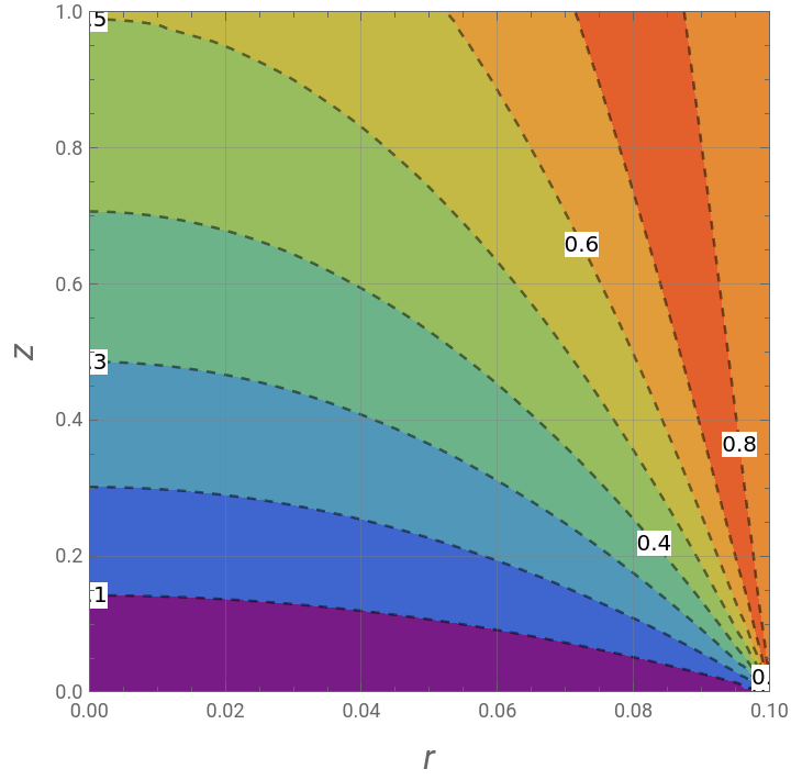

Superposing our Mathematica result and its counterpart using Matlab. We get Figure 9 of Ref. 2.
Result obtained using Matlab
Computation of mixing-cup concentration
References
References
◼
◼
[2] A.-H. Soares, L. de Sousa Santos, H. Binous, A. A. Shaikh, and A. Bellagi, Exploring tubular steady-state laminar flow reactors with orthogonal collocation, Comput. Appl. Eng. Educ. (2024), e22795. https://doi.org/10.1002/cae.22795
CITE THIS NOTEBOOK
CITE THIS NOTEBOOK
Fogler's adiabatic laminar flow reactor
by André von-Held Soares, Lizandro de Sousa Santos, Housam Binous, Abdullah A. Shaikh and Ahmed Bellagi
Wolfram Community, STAFF PICKS, September 14, 2024
https://community.wolfram.com/groups/-/m/t/3274313
by André von-Held Soares, Lizandro de Sousa Santos, Housam Binous, Abdullah A. Shaikh and Ahmed Bellagi
Wolfram Community, STAFF PICKS, September 14, 2024
https://community.wolfram.com/groups/-/m/t/3274313