ABSTRACT (original book): This book provides General Relativity problems to be tackled both analytically and symbolically-numerically with the Mathematica software. In the first case, the reader is guided in setting up the appropriate solutions. In the second case, the reader is provided with very illustrative notebooks to carry out the steps necessary to solve a General Relativity problem. These include the calculation of the Christoffel symbols, Riemann, Ricci, Einstein and energy-momentum tensors, as well as the resolution of the field equations of General Relativity in different astrophysical/cosmological contexts, with and without the introduction of a cosmological constant. This study guide should be used alongside existing textbooks to provide additional learning and engagement opportunities for advanced undergraduate and graduate students in physics and astrophysics taking courses on general relativity. It may also be of interest to mathematics students interested in celestial mechanics and space sciences. CITATION (original book): Vittorio, N. (2025). General Relativity: Analytic and Symbolic Problems with Mathematica (1st ed.). CRC Press. ISBN: 9781032674858. https://doi.org/10.1201/9781032674858
Amazon: https://amzn.eu/d/22exs2v
Amazon: https://amzn.eu/d/22exs2v
Introduction
Introduction
This book is based on the results of a teaching experiment I conducted during the course of Relativity and Cosmology for first-year students of the Master degree in Physics at the University of Rome “Tor Vergata”. The educational objectives of the course were to present in a coherent way the basics of General Relativity and its applications. The class group I had to deal with was rather inhomogeneous, both in terms of initial education (most of the students had a Bachelor in Physics, but others had a Bachelor in Mathematics) and in terms of interests (some students were more taken by the formal aspects of the theory, others were more attracted by the experimental results and the astrophysical applications). None of the students were exposed to courses on differential geometry. To overcome all these differences, I tried to favor a practical approach. In particular,
- I organized the lectures by reducing when possible the abstract formalization and by organizing them in terms of problems to be solved, even to address specific analytical derivations. I found that this way the students’ attention was captured more easily and that it was easier to connect different problems and topics.
-Once I introduced the meaning and use of all the necessary geometric objects, I used the Mathematica software, free for all students, to perform symbolic calculations. The advantage of this approach is to avoid long and often boring mathematical steps, and to better focus on the physics of the problems.
I found the results of this experiment quite encouraging. The formal aspects of tensor calculus were more easily grasped by the students by writing numerical codes. For example, deriving Christoffel symbols or writing the Riemann tensor for different space-time metrics were tackled quite easily by all the students in the class group. The advantage of this approach is that it allows students to directly build and manage all the different geometric objects of interest for the course, without having to use software available on the net as black boxes. Furthermore, being in a computer lab encouraged collaboration among all students and created a good team spirit in the class group. Several Mathematica codes were designed to produce plots of different theoretical situations (e.g., the perihelion advance of Mercury or the shape of the horizons of a Kerr black hole). I found particularly rewarding for students to produce these plots themselves, rather than finding similar ones printed in a book.
- I organized the lectures by reducing when possible the abstract formalization and by organizing them in terms of problems to be solved, even to address specific analytical derivations. I found that this way the students’ attention was captured more easily and that it was easier to connect different problems and topics.
-Once I introduced the meaning and use of all the necessary geometric objects, I used the Mathematica software, free for all students, to perform symbolic calculations. The advantage of this approach is to avoid long and often boring mathematical steps, and to better focus on the physics of the problems.
I found the results of this experiment quite encouraging. The formal aspects of tensor calculus were more easily grasped by the students by writing numerical codes. For example, deriving Christoffel symbols or writing the Riemann tensor for different space-time metrics were tackled quite easily by all the students in the class group. The advantage of this approach is that it allows students to directly build and manage all the different geometric objects of interest for the course, without having to use software available on the net as black boxes. Furthermore, being in a computer lab encouraged collaboration among all students and created a good team spirit in the class group. Several Mathematica codes were designed to produce plots of different theoretical situations (e.g., the perihelion advance of Mercury or the shape of the horizons of a Kerr black hole). I found particularly rewarding for students to produce these plots themselves, rather than finding similar ones printed in a book.
Below, you’ll find illustrative examples from three key chapters.
Chapter 9 (Classical tests of General Relativity)
Chapter 9 (Classical tests of General Relativity)
This Chapter focuses on the classical tests of General Relativity, including planetary motion, the deflection of light rays, gravitational lensing, and the Shapiro time delay. It is structured around problems with analytical solutions and includes Mathematica notebooks for symbolic calculations.Section 9.1 covers the orbital motion of a test particle in a Schwarzschild space-time, described using the variable [ϕ(s)]. The corresponding equation of motion is expressed as , where m is the mass of the central body in geometrical units and h is the angular momentum of a test particle per unit mass. The initial five problems focus on: i) Deriving the equation of motion (9.1); ii) Using the weak field limit to determine the classical solution (9.2); iii) Evaluating the relative significance of the 3m and terms within the solar planetary system (9.3); iv) Deriving the perturbative solution u[ϕ] = [A+ϵ (A + )] - ϵ Cos[ 2ϕ] + B Cos[(1-ϵ) ϕ] of the equation of motion (9.4); v) Finding the precession of the planet’s periastron (9.5). These problems can be solved by the teacher on the blackboard, assigned as homework to students, or discuss in the class by a group of them. In any case, the book provides specific hints, followed by full solutions that are shown and discussed. Only after this, I ask the students to reproduce the “shift of the periastron” using this Mathematica code.
u[ϕ(s)]=
-1
r
u''+u=m/+3
2
h
2
mu
2
u
m/
2
h
2
B
2A
2
B
6A
As shown in Problem 9.2, the classical solution for the elliptical motion of a test particle around a point mass is given by Eq.(I8)
In[]:=
u0[ϕ_]:=A+BCos[ϕ]
Let’s choose for graphical purposes the following values
In[]:=
A=1;
In[]:=
B=.5;
In[]:=
Δϕ=1.85;
The corresponding Cartesian coordinates of the ellipse are
In[]:=
x0[ϕ_]:=
Cos[ϕ+Δϕ]
u0[ϕ]
In[]:=
y0[ϕ_]:=
Sin[ϕ+Δϕ]
u0[ϕ]
Plot the solution for a single round from 14π to 16π, values chosen only for graphical reasons
In[]:=
P0=ParametricPlot[{x0[ϕ],y0[ϕ]},{ϕ,14π,16π},PlotRange{{-2,2},{-2,2}},AspectRatio1,AxesFalse,PlotStyle{{Black,DotDashed,Thickness[0.0075]}}];
Indicate the point mass as a dot at the origin of the Cartesian frame
In[]:=
PM=Graphics[Disk[{0,0},.1]];
The position of the periastron is obtained by maximizing u0[ϕ]
In[]:=
ϕmax0=Maximize[{u0[ϕ],14π≤ϕ≤16π},ϕ][[2,1,2]];
Let’s indicated with a gray dot
In[]:=
Pastro0=Graphics[{Gray,Disk[{x0[ϕmax0],y0[ϕmax0]},.1]}];
and join it with the central mass with a dashed line
In[]:=
L0=Graphics[{Thickness[0.01],Dashed,Line[{{0,0},{x0[ϕmax0],y0[ϕmax0]}}]}];
As a result, one gets
In[]:=
P0dots=Show[P0,Pastro0,L0,PM]
Out[]=
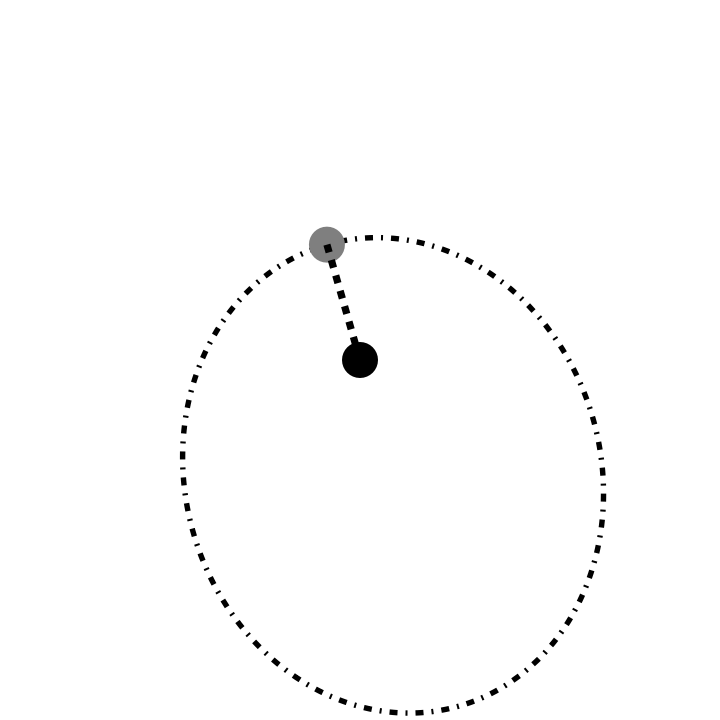
The relativistic solution is given by Eq.(9.2)
In[]:=
u[ϕ_]:=A+ϵA+-ϵCos[2ϕ]+BCos[(1-ϵ)ϕ]
2
B
2A
2
B
6A
Let’s use the same values of A and B used for the classical case, with ϵ=0.04
In[]:=
A=1;
In[]:=
B=.5;
In[]:=
ϵ=0.04;
The corresponding Cartesian coordinates of the ellipse are
In[]:=
x[ϕ_]:=
Cos[ϕ]
u[ϕ]
In[]:=
y[ϕ_]:=
Sin[ϕ]
u[ϕ]
Let’s plot the relativistic solution for a single round from 14π to 16π
In[]:=
P1=ParametricPlot[{x[ϕ],y[ϕ]},{ϕ,14π,16π},PlotRange{{-2,2},{-2,2}},AspectRatio1,AxesFalse,PlotStyle{{Black,Thickness[0.015]}}];
The position of the periastron is now obtained by maximizing u[ϕ]
In[]:=
ϕmax1=Maximize[{u[ϕ],14π≤ϕ≤16π},ϕ][[2,1,2]];
Let’s indicated it with a gray dot
In[]:=
Pastro1=Graphics[{Gray,Disk[{x[ϕmax1],y[ϕmax1]},.1]}];
and join it with the central mass with a dashed line
In[]:=
L1=Graphics[{Thickness[0.01],Dashed,Line[{{0,0},{x[ϕmax1],y[ϕmax1]}}]}];
As a result, one gets
In[]:=
P1dots=Show[P1,Pastro1,L1,PM]
Out[]=

If we compare the classical with the relativistic result we get
In[]:=
Show[P0dots,P1dots]
Out[]=

The relativistic solution is similar to an ellipse, but unlike the classical case the orbit is not closed. Clearly there is an analogous situation for the next orbit that goes from 18π to 20π
The position of the periastron is again obtained by maximizing u[ϕ]
Let’s indicated it with a gray dot
and join it with the central mass with a dashed line
As a result, one gets
Let’s now compare the round from 14π to 16π with the one from 18π to 20π. One gets the following
The orbit is still open and the periastron moved wrt to the previous position in the same direction of the orbital motion. At this point, let’s plot the trajectory of the test-particle after sim 25 rounds around the central body
This is the so-called rosette orbits: the orbits are open ellipses, with their semi-axis rotating in the equatorial plane. To show more explicit the periastron precession lets plot together the rosette orbits with the two round shown above
Chapter 10 (Linearized Gravity)
Chapter 10 (Linearized Gravity)
Then, the metric of the space-time in the linearized gravity regime is given by
Clearly the inverse of the Minkowski metric is the Minkowski metric. Then, to first order, the Christoffel symbols are written in the following ways
Next, let’s consider the time-space component of the field equations
reinforcing the point that Ψ, and then Φ, are time independent quantities. So, in conclusions, the field equations for gauge-invariant scalar modes provides the following metric
Chapter 12 (Schwarzschild Black Holes)
Chapter 12 (Schwarzschild Black Holes)
The metric tensor and its inverse write
The Christoffel symbols are evaluated according to Eq.(3.4)
The derivatives of the Christoffel symbols wrt the coordinates are given by
The Kretschmann invariant is given by the inner product of the Riemann tensor with itself, saturating all the four indices.
CITE THIS NOTEBOOK
CITE THIS NOTEBOOK
General relativity: analytic and symbolic problems with Mathematica
by Nicola Vittorio
Wolfram Community, STAFF PICKS, September 10, 2025
https://community.wolfram.com/groups/-/m/t/3543806
by Nicola Vittorio
Wolfram Community, STAFF PICKS, September 10, 2025
https://community.wolfram.com/groups/-/m/t/3543806