Ordinary Turing Machines are implemented on infinite 1D tapes. This project investigates and explores the behavior of Turing Machines on finite cyclic graphs . The graphs investigated are the circular Cyclic Graph, a Torus and the Sierpinski Network. This post demonstrates that the Sierpinski network exhibits the most complex and varied behavior.
Introduction to Turing Machines on Graphs
Introduction to Turing Machines on Graphs
An ordinary Turing Machine consists of a linear tape divided into cells, where each cell consists of a color and a state as indicated by the machines head. The machine’s head moves left and right along the tape, updating the state and color based on specified transition rules. In a graph-based Turing machine, instead of a linear tape, the machine’s computation takes place on a network of vertices and edges. The Turing Machine on a graph moves from node to node, following the edges based on the current state and the symbol it encounters. Whereas a traditional Turing Machine only move left and right, the Turing Machine on a Graph can move in any direction, only constrained by the number of adjacent edges. In this post the notation (state, color)-TM I used to refer to a specific Turing Machine. For example, a 1-state, 2-color Turing Machine is denoted as: (1,2)-TM.
Rule Definition
Rule Definition
The number of possible rules for a given Turing Machine is determined by the number of states, colors, and edges (if it is a graph). The total number of possible rules is given as:
(edges states colors)^(states colors);
For example a 1-state, 2-color linear tape (2-edges) there 16 number of rules:
In[]:=
(2×1×2)^(1×2)
Out[]=
16
For a 2-state, 2-color graph Turing Machine with 4 edges there are 65536 number of rules:
In[]:=
(4×2×2)^(2×2)
Out[]=
65536
Given the number of states, colors, and edges in a Turing Machine the rules governing a specific Turing Machine is defined in the following function:
In[]:=
netTMRules[state_Integer, color_Integer, edges_Integer, ruleNr_Integer] := Thread[Tuples[{Range[1, state], Range[0, color - 1]}] -> Tuples[Tuples[{Range[1, state], Range[0, color - 1], Range[1, edges]}], {state*color}][[ruleNr]]]
The format for the rules follows the format:
{State, Color} -> {State, Color, Next edge to follow}.
{State, Color} -> {State, Color, Next edge to follow}.
For example for 2-states, 2-colors and 2 edges we have Rule 441 specified as:
In[]:=
netTMRules[2,2,2,441]
Out[]=
{{1,0}{1,0,1},{1,1}{2,1,1},{2,0}{2,1,2},{2,1}{1,0,1}}
Example of a Turing Machine Evolution on a Graph
Example of a Turing Machine Evolution on a Graph
The simplest possible graph-based Turing Machine is the cyclic graph. Essentially, it is a linear Turing Machine where the two ends of the tape are glued together. A small cycle Turing Machine with 4 nodes is shown here to illustrate the analysis that will later be performed on more complex graphs.
In[]:=
{adjacencyList,edges,verticies}=cyclicGraph[4,1];nrEdges=2;inputGraph=adjacencyList;
In[]:=
SimpleGraph[Graph[verticies,edges],VertexLabels->Automatic]
Out[]=
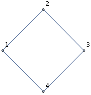
The Turing Machine starts with a graph in a given initial conditions indicating the color of each node and the position of the head.
The machine under investigation starts with a colored node at vertex three and all other cells being white.
The machine under investigation starts with a colored node at vertex three and all other cells being white.
In[]:=
startVertex=3;intialState={1,ReplacePart[Table[0,Length[inputGraph]],startVertex->1],startVertex}
Out[]=
{1,{0,0,1,0},3}
With a 1-state, 2-color Turing machine Rule number 14 gives the following behaviour.
In[]:=
nrStates=1;nrColors=2;nrIterations=16;nrRule=14;
In[]:=
inputRule=NetTMRules[nrStates,nrColors,nrEdges,nrRule]
Out[]=
{{1,0}{1,1,2},{1,1}{1,0,2}}
In[]:=
outEvolution=NetTMEvolveList[inputRule,inputGraph,intialState,nrIterations];
In[]:=
ListAnimate[Table[NetTMGraphics[SimpleGraph[Graph[verticies,edges]],l],{l,outEvolution}]]
Out[]=
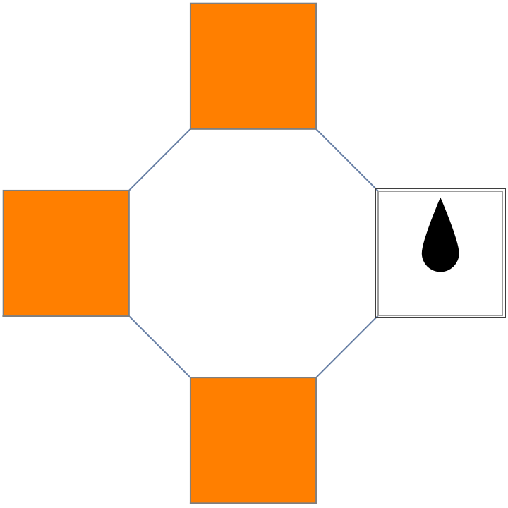
The Rule number 14 (1,2)-Turing Machine travels around the cyclic graph changing the color for each iteration. The behavior of the Turing Machine can more conveniently be displayed by flattening out the graph to a 1D grid ordered by vertex number. This can be generalized for any graph type.
In[]:=
EvolutionRulePlot[nrStates,nrColors,outEvolution]
Out[]=
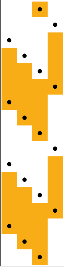
In the Turing Machine Plot above it is easier to see that the Turing Machine repeats itself every 8 steps. When running for many iterations the Turing Machine plot will be split into multiple pallets to make the visualization easier.
The cyclic behavior of Rule 14 can also be illustrated using a state Transition diagram.
The cyclic behavior of Rule 14 can also be illustrated using a state Transition diagram.
In[]:=
netTransitionDiagram[nrRule,inputGraph,nrStates,nrColors,nrEdges,nrIterations]
Out[]=
14 |
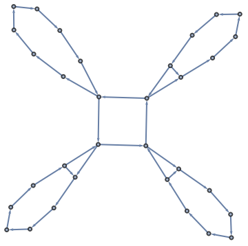
The state transition diagram shows how to Turing Machine transitions from one state to the next eventually looping around to the same state and repeating. For example the first state transition in our current example is {1,{0,0,1,0},3}->{1,{0,0,0,0},5}. The state diagram consist of the state transitions for all possible vertex starting positions, states, and colors which is why there are multiple loops in each diagram.
In this post we will also be analyzing the Turing Machines behavior based on the edge distance from the starting vertex points. For the cycle graph of 4 nodes the max distance from the starting point is 2:
In this post we will also be analyzing the Turing Machines behavior based on the edge distance from the starting vertex points. For the cycle graph of 4 nodes the max distance from the starting point is 2:
Cyclic Graph Turing Machine
Cyclic Graph Turing Machine
This Chapter shows the results for the cyclic graph Turing Machine now expanded to 7 vertices and multiple rules.
CyclicGraph[7]: 1-State and 2-Color Turing Machines
CyclicGraph[7]: 1-State and 2-Color Turing Machines
Of the 16 possible rules for the (1,2)-Turing Machine, Rules 9, 10, 13 and 14 are worth highlighting. The Turing Machine Plot, state transition diagram and graph distance plot are show bellow.
The four rules all show a repetitive pattern. Rule number 9 and 13 (and 10 and 13) are almost mirror images of each other. However, there is a small difference in the traversal which can be seen in the difference between the edge distance diagram of 10 and 13. Rule number 10 and 13 both make a sidestep before continuing to cycle around the graph.
Besides rule 9, 10, 13, and 14 the other rules for the (1,2) Turing Machine on a cycle graph show only simple repetitive behavior e.g., bouncing back and forth between two states. Despite their simplicity, the state Transitions diagrams can still appear quite complex for even simplest scenarios.
Besides rule 9, 10, 13, and 14 the other rules for the (1,2) Turing Machine on a cycle graph show only simple repetitive behavior e.g., bouncing back and forth between two states. Despite their simplicity, the state Transitions diagrams can still appear quite complex for even simplest scenarios.
CyclicGraph[7]: 2-State and 2-Color Turing Machines
CyclicGraph[7]: 2-State and 2-Color Turing Machines
To get more complex Turing Machines we increase the number of states to 2.
For the 2-state and 2-color diagram cycle graph the following number of possible rules:
I have sifted through all of them and found that most of them have simple repetitive behavior. For example, bouncing back and forth between two nodes. The Rules 372, 316 and 3037 have been found to display more complexity repetitive patterns.
In the above figure each panel is a continuation of the Turing Machine for the respective rule. We see that there is a long repetitive patter in each of the Turing Machines. The repetitive patter is also evident by looking at the graph distance of the Turing Machine head as shown below.
The pattern for the rules 372, 316 and 3037 starts repeating itself after the first 54, 189 and 22 iterations respectively.
Some other interesting rules to explore for the (2,2)-TM Cycle graph would be rule number: 1372, 3417, 1404, 2454, 1353, 3953, 2206, 470
Torus Graph Turing Machine
Torus Graph Turing Machine
This Chapter investigates the Turing Machine on a Torus. The Torus is formed by labeling all the vertices on a 2D grid then merging the edges on the top to bottom and side to side. By merging the edges, we create a cyclic Turing Machine that wraps around itself just like the cycle graph.
The Torus formed by the 3x7 grid is created and shown in 1D below. I have also run the simulations with other grid sizes of various permutations, however I did not find that small changes had an impact on the Turing Machine. When running on much larger grids e.g. 30x70 the results are substantially different.
Torus[3,7] - 1-State and 2-Color Turing Machines
Torus[3,7] - 1-State and 2-Color Turing Machines
For the 1-state and 2-color Torus there are the following number of possible rules:
Like the 1-state, 2-color cyclic graph most of the 64 rules for the torus are mirror images of each or otherwise simple repetitive behavior. Here is an example of a few of the more interesting Rules.
Like with the (1,2) Cycle Graph Turing Machine we see that rule 43 and 44 are near mirror images of each other however they display different state transition diagrams.
The pattern for the rules 43, 44, 50 starts repeating itself after the first 45, 45 and 49 iterations respectively.
Torus(3x7) - 2-State and 2-Color Turing Machines
Torus(3x7) - 2-State and 2-Color Turing Machines
The same Torus formed by the 3x7 grid is used in this section. Now we increase the complexity to 2-states. For the 2-state and 2-color Torus there are the following number of possible rules:
The number of rules has grown exponentially. During the project I have run the Turing Machine for about half the rules and found some that exhibit quite complex behavior.
We see that the patter are much more complex, however they still display a ceratin repetitive cycling.
Some other interesting rules to explore would be: {3403, 2753, 3803, 63002, 19231, 19291, 23281, 31051, 31201, 63811}
Some other interesting rules to explore would be: {3403, 2753, 3803, 63002, 19231, 19291, 23281, 31051, 31201, 63811}
Large Torus (30x70) - 2-State and 2-Color Turing Machines
Large Torus (30x70) - 2-State and 2-Color Turing Machines
With a larger system the head of the Turing Machine can travel much further from the starting node before wrapping around to the same position again. Using the same rules as in the above section we use a larger torus of 30 by 70 nodes.
The graph distance shown above for rule 23,281 looks like a stochastic behavior and could have been produced by stock price data. The perceived randomness from Rule 23,281 is amazing considering that it is the result of a fully deterministic process that repeats cyclically.
Rule 19,291 on the other hand cycles regularly through the entire torus in the beginning and then begins a more chaotic cycle.
The Turing Machine plot for the two rules is shown below. Both graphs start out with all the nodes colored white and as the Turing Machine travels along the edges, the nodes are gradually colored orange. For a further investigation it would be interesting highlight the edges on the Torus that the Turing Machine travels around.
Rule 19,291 on the other hand cycles regularly through the entire torus in the beginning and then begins a more chaotic cycle.
The Turing Machine plot for the two rules is shown below. Both graphs start out with all the nodes colored white and as the Turing Machine travels along the edges, the nodes are gradually colored orange. For a further investigation it would be interesting highlight the edges on the Torus that the Turing Machine travels around.
Turing Machine On Sierpinski Graph
Turing Machine On Sierpinski Graph
In this Chapter we generate the Turing Machine on the Sierpinski Network. The traditional Sierpinski graph has the property that the corners of the vertices only have three edges while the rest of the nodes have four. To implement the Turing Machine on the Sierpinski graph we need to deal with the corner effects. In this project we have generated a Sierpinski graph by taking another Sierpinski graph of one degree smaller merging the three corners. The two Sierpinski that are joined are shown below.
By merging the three corners of the two Sierpinski’s we get a Cyclic Sierpinski graph that wraps around and has all vertices with four edges.
With the Torus and the Cycle graph there is a natural left, right, up, and down that can be defined. The geometry of the Sierpinski makes the decision of which node is up and down more difficult. During the project we explored various options from simply numbering the vertices to treating each neighboring triangle as a ternary diagram. In the end we decided to assign a coloring to each of the edges. The decision of left vs right thus becomes red, yellow, purple, orange.
The geometry of the Sierpinski graph has been generalized to any degree however the rest of this Chapter we will focus on the smallest Sierpinski of degree-1 shown below.
The geometry of the Sierpinski graph has been generalized to any degree however the rest of this Chapter we will focus on the smallest Sierpinski of degree-1 shown below.
Sierpinski Network with 1-State and 2-Color Turing Machines
Sierpinski Network with 1-State and 2-Color Turing Machines
Immediately, we see that the Sierpinski (1,2)-Turing Machine has a more complex and varied behavior as compared to what we saw for the Cycle graph and the Torus. The state transition diagram especially show a different structure which wasn’t observed in any of the underlying rules for the Torus.
Sierpinski Network with 2-State and 2-Color Turing Machines
Sierpinski Network with 2-State and 2-Color Turing Machines
Like with the Cycle graph and the Torus we now investigate the 2-state and 2-color Turing Machine for the Sierpinski network.
With the above Turing Machines the use of the state transition diagram become much too big to display.
Looking at Rule number 50 001 we see it has a repetitive structure in the edge distance plot. The coloring in the Turing Machine plot for Rule 50,001 is quite different from most of the other Turing Machines explored being mostly colored orange with some whole of white here and there.
With Rule number 59,656 there is not any obvious repetitive behavior. I found from running it for 10K iterations that there is a repetitive cycle that emerges after 5326 iterations.
The complexity of theses Turing Machines starts to exceed what can be discerned from visual inspection. One test we can perform to understand the behavior is to see if the Turing Machine visits all nodes (completes a Hamiltonian cycle).
From the below code we see that both the Turing machines do in fact visit all nodes 18 within the 1000 iterations.
Looking at Rule number 50 001 we see it has a repetitive structure in the edge distance plot. The coloring in the Turing Machine plot for Rule 50,001 is quite different from most of the other Turing Machines explored being mostly colored orange with some whole of white here and there.
With Rule number 59,656 there is not any obvious repetitive behavior. I found from running it for 10K iterations that there is a repetitive cycle that emerges after 5326 iterations.
The complexity of theses Turing Machines starts to exceed what can be discerned from visual inspection. One test we can perform to understand the behavior is to see if the Turing Machine visits all nodes (completes a Hamiltonian cycle).
From the below code we see that both the Turing machines do in fact visit all nodes 18 within the 1000 iterations.
Some other rules worth exploring are Rules numbers: {18785, 51736, 60181, 40051, 59446, 48706, 40516, 60166, 59656}
Extended Sierpinski Network with 2-State and 2-Color Turing Machines
Extended Sierpinski Network with 2-State and 2-Color Turing Machines
To get the image used for the title page the (2,2)-Turing Machine with Rule 59,656 is simulated for 5000 iterations and shown.
Bonus: Machine Music
Bonus: Machine Music
One area explored during the project was making exploring the repetitive structure of the Turing Machine by converting them into sound. In this Chapter I use the Sierpinski network for the (1,2) Turing Machine.
To generate a pleasant melody I assign each node in the network to a note in the C Major scale. We start the scale one octave below middle C then we iteratively adding more keys over multiple octaves.
Here is the melody for Rule 59 and 41. The corresponding Turing Machine plot is shown below.
The rhythm used for these examples very monotonous since each key is pressed down on every beat. The algorithm could be improved by having the keys only being pressed down a single time when the node change from white to orange. This would generate a much more dynamical and musical composition.
Future Work
Future Work
In this project I have only scratched the surface for the exploration of Turing Machines on Graphs.
◼
The cyclic behavior of the Turing Machines studied needs to be investigated further to understand their underlying functional behavior. For example, if a rule is a binary counter or if it cycles through a set of primary numbers.
◼
It needs to be determined if the coloring scheme used for the Sierpinski graph is isomorphic and what the impact would be on the results for the Turing Machine if it isn’t.
◼
There are endless possibilities of various graphs that could be explored. For future work, I would propose that the Hexagonal Torus and Petersen graphs be explored as examples of graphs with a valence of 3.
Conclusion
Conclusion
This post has investigated the 1-state/2-state and 2-color Turing Machines on finite graphs. The graphs used were the 1D Cyclic graph, the Torus and the cyclic Sierpinski network. It was found that the cyclic Sierpinski network showed more complex patters for the (1,2)-Turing Machine than the cycle graph and Torus. Similarly, the (2, 2)-TM Sierpinski network showed more complexity as compared to (2,2)-Turing Machine on the Torus and Cycle Graph.
However, when running the Turing Machine on a larger Torus (30x70) with more room for the head to move around, I found that there was a stochastic looking behavior that arises. The perceived stochastic behaviour is impressive considering that it is fully deterministic and follows a regular cyclic patter.
The Turing Machines on the Sierpinski network are worth further exploration. Specifically, it is necessary to prove that the coloring scheme used for the Sierpinski network is isomorphic. An deeper analysis should also be performed on the Sierpinski network of higher degree and the Torus with more nodes.
However, when running the Turing Machine on a larger Torus (30x70) with more room for the head to move around, I found that there was a stochastic looking behavior that arises. The perceived stochastic behaviour is impressive considering that it is fully deterministic and follows a regular cyclic patter.
The Turing Machines on the Sierpinski network are worth further exploration. Specifically, it is necessary to prove that the coloring scheme used for the Sierpinski network is isomorphic. An deeper analysis should also be performed on the Sierpinski network of higher degree and the Torus with more nodes.
Keywords
Keywords
◼
Turing Machines
◼
Networks
◼
Graphs
◼
Sierpinski
Acknowledgment
Acknowledgment
◼
To my mentors Robert Nachbar and Alejandra Ortzi for guiding me through the project. Specifically, Alejandra came up with the idea for coloring the Sierpinski graph to determine the coordinate system and Robert came up with the generalized geometry for the cyclic Sierpinski graph.
◼
To Stephen Wolfram for the initial project idea and discussions on how to best analyze the results.
◼
To all the Wolfram staff who helped organize the 2023 Wolfram Summer School.
References
References
◼
Stephen Wolfram, A New Kind Of Science, Wolfram Media (2002). ISBN: 1-57955-008-8
◼
Stocke, Joseph, Turing machine evolution on graphs using principles of multiway computation, 2023
CITE THIS NOTEBOOK
CITE THIS NOTEBOOK
Turing machines on graphs
by Stefan Graham
Wolfram Community, STAFF PICKS, July 12, 2023
https://community.wolfram.com/groups/-/m/t/2959123
by Stefan Graham
Wolfram Community, STAFF PICKS, July 12, 2023
https://community.wolfram.com/groups/-/m/t/2959123