Liquid chromatography is a common technique in analytical chemistry used to identify and quantify chemical species in a mixture. The mixture is injected at the inlet of a chromatographic column and a liquid mobile phase (the solvent) allows their elution. The liquid chromatography technique is based on the difference in adsorption of the chemicals on a solid stationary phase or adsorbent. Hence, different chemical species will elute at different retention times.
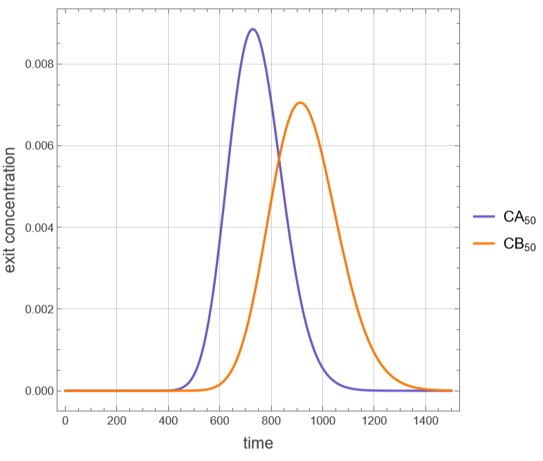
In this notebook, two components (A and B) are separated by liquid chromatography using the stagewise model. This model considers the chromatographic column to be a series of 50 well-mixed stirred tanks or 50 perfect equilibrium stages. Linear adsorption isotherms with equilibrium constants are assumed for this stagewise model. The two peaks at the exit of the column are plotted. These peaks are symmetric because of the linear equilibrium hypothesis. The order of elution of the two components depends on the relative values of their equilibrium constants, which can be varied. Due to dispersion, peaks get broader and smaller for larger elution times.
In this notebook, two components (A and B) are separated by liquid chromatography using the stagewise model. This model considers the chromatographic column to be a series of 50 well-mixed stirred tanks or 50 perfect equilibrium stages. Linear adsorption isotherms with equilibrium constants are assumed for this stagewise model. The two peaks at the exit of the column are plotted. These peaks are symmetric because of the linear equilibrium hypothesis. The order of elution of the two components depends on the relative values of their equilibrium constants, which can be varied. Due to dispersion, peaks get broader and smaller for larger elution times.
Base case - sloppy separation
Base case - sloppy separation
Equilibrium constants
KA=0.9;KB=1.3;
Total volume
V
tot
50 well-mixed stirred tanks or 50 perfect equilibrium stages
NS=50;
Stage volume
V
stage
V
tot
Volumetric flow rate
L=0.4;
Void fraction
ϵ=0.4;
Column length
Lbed=25;
Column diameter
Dc=4;
In[]:=
eq[i_]:=D[[t],{t,1}]L([t]-[t])ϵ+(1-ϵ)KA;eq2[i_]:=D[[t],{t,1}]L([t]-[t])ϵ+(1-ϵ)KB;eqn=Table[eq[i],{i,1,50}];
CA
i
CA
i-1
CA
i
V
stage
V
stage
CB
i
CB
i-1
CB
i
V
stage
V
stage
In[]:=
initialCond=Table[[0]0,{i,1,50}];sys=Flatten[Join[eqn,initialCond]];Unknown=Table[,{i,1,50}];eqn2=Table[eq2[i],{i,1,50}];initialCond2=Table[[0]0,{i,1,50}];sys2=Flatten[Join[eqn2,initialCond2]];Unkn2=Table[,{i,1,50}];
CA
i
CA
i
CB
i
CB
i
In[]:=
CA
0
CA
init
CA
init
CB
0
CB
init
CB
init
In[]:=
sol1=NDSolve[sys,Unknown,{t,0,5000}];sol2=NDSolve[sys2,Unkn2,{t,0,3000}];
plt2=Plot{Evaluate[[t]]/.sol1,Evaluate[[t]]/.sol2},{t,0,1500},
CA
50
CB
50
Out[]=
Resolution (Rs) separation criterion
Resolution (Rs) separation criterion
Match the upper t-limit used in NDSolve/Plot for this case
tmax=2000;
In[]:=
cA[t_]:=Evaluate[[t]]/.sol1[[1]]cB[t_]:=Evaluate[[t]]/.sol2[[1]]
CA
50
CB
50
Zeroth moment: area under each peak
areaA=NIntegrate[cA[t],{t,0,tmax}];areaB=NIntegrate[cB[t],{t,0,tmax}];
First moment: retention time (mean elution time)
tRA=NIntegrate[t*cA[t],{t,0,tmax}]/areaA;tRB=NIntegrate[t*cB[t],{t,0,tmax}]/areaB;
Second central moment: variance->sigma
varA=NIntegrate[(t-tRA)^2*cA[t],{t,0,tmax}]/areaA;varB=NIntegrate[(t-tRB)^2*cB[t],{t,0,tmax}]/areaB;sigmaA=Sqrt[varA];sigmaB=Sqrt[varB];
Baseline peak width, Gaussian approx: w=4*sigma
wA=4*sigmaA;wB=4*sigmaB;
Resolution
Rs=2*(tRB-tRA)/(wA+wB);Print["Retention time A = ",NumberForm[tRA,5]];Print["Retention time B = ",NumberForm[tRB,5]];Print["Peak width A (4σ) = ",NumberForm[wA,5]];Print["Peak width B (4σ) = ",NumberForm[wB,5]];Print["Resolution Rs = ",NumberForm[Rs,4]];
Retention time A = 743.27
Retention time B = 931.77
Peak width A (4σ) = 417.79
Peak width B (4σ) = 524.38
Resolution Rs = 0.4001
Base case with a temperature gradient along the column
Base case with a temperature gradient along the column
The column is no longer isothermal: a linear temperature profile T(z) is imposed along the bed, from Tin at the inlet (z=0) to Tout at the outlet (z=1). Each of the NS stages of the plate model represents a thin slice of the bed, so stage i sits at position z=(i-1)/(NS-1) and has its own local temperature T[i]. The equilibrium constants KA and KB are no longer fixed numbers: they follow a van't Hoff-type law, KA(T) = KA0 Exp[-(ΔHA/R)(1/T-1/Tref)], and similarly for KB, so KA[i] and KB[i] are evaluated at the local stage temperature T[i]. KA0 and KB0 equal the original constant values (0.9 and 1.3), so setting Tin = Tout reduces this exactly to the original isothermal base case.
Base case geometry and operating conditions - same as the original base case
L=0.4;(*volumetricflowrate*)eps=0.4;(*voidfraction*)Dc=4;(*columndiameter*)Lbed=25;(*columnlength*)Vtot=Lbed*Pi*Dc*Dc/4.;(*totalvolume*)NS=50;(*numberofequilibriumstages*)Vstage=Vtot/NS;(*stagevolume*)
In[]:=
Clear[KA,KB]
Temperature gradient along the column and temperature-dependent equilibrium constants
Column inlet temperature, K
Tin=298.15;
Column outlet temperature, K - the column is heated along its length
Tout=348.15;
Reference temperature at which KA0 and KB0 were measured
Tref=298.15;
Ideal gas constant, J/(mol K)
Rgas=8.314;
KA at Tref - same value as the original isothermal base case
KA0=0.9;
KB at Tref - same value as the original isothermal base case
KB0=1.3;
Adsorption enthalpy of A, J/mol (exothermic, so KA falls as T rises)
dHA=-35000.;
Adsorption enthalpy of B, J/mol
dHB=-5000;
z: fractional position along the bed, 0=inlet, 1=outlet
Tpos[z_]:=Tin+(Tout-Tin)*z;
Temperature seen by stage i
T[i_]:=Tpos[(i-1)/(NS-1)];
van’t Hoff law for A
KA[i_]:=KA0*Exp[-(dHA/Rgas)*(1/T[i]-1/Tref)];
van’t Hoff law for B
Stage mass balances - same form as the original base case, but KA and KB are replaced by the local, temperature-dependent KA[i] and KB[i]
Resolution (Rs) separation criterion
Resolution (Rs) separation criterion
Match the upper t-limit used in NDSolve/Plot for this case
Zeroth moment:area under each peak
First moment:retention time (mean elution time)
Second central moment: variance->sigma
Baseline peak width, Gaussian approx: w=4*sigma
Resolution
Discussion
Discussion
Adding a temperature gradient changes the separation noticeably. In the isothermal base case both KA and KB are fixed at their Tref values (0.9 and 1.3) and the column elutes A at t = 743.27 and B at t = 931.77, giving a resolution of only Rs = 0.4001 - the two peaks are badly overlapped. With the column running from 298.15 K at the inlet to 358.15 K at the outlet, both peaks come out earlier (tRA = 493.37, tRB = 847.21) and the resolution nearly triples, to Rs = 0.931. Both retention times drop because adsorption is exothermic (ΔHA, ΔHB < 0): most of the bed now sits above Tref, so the stage-averaged KA and KB are both lower than their isothermal, Tref values, and a lower K means less time held up in the stationary phase.
The resolution gain is the more interesting effect, and it is not simply a byproduct of faster elution: KA and KB do not soften at the same rate as the column warms up, because ΔHA is more negative than ΔHB (-35000 versus -5000 J/mol). A's equilibrium constant is therefore more temperature-sensitive than B's, so the selectivity KB/KA drifts along the length of the column instead of staying fixed as it does in the isothermal case. For this particular choice of enthalpies and end-point temperatures that drift happens to widen the gap between the two peaks even as both move earlier - the same mechanism gradient elution exploits by varying solvent strength, but implemented here through a temperature profile acting on the equilibrium constants instead.
Column temperature gradient is a real, tunable separation lever, similar in spirit to solvent gradient elution.The sign and relative size of ΔHA and ΔHB for the specific pair of analytes play an important role. Here warming the column toward the outlet happened to help both speed and resolution because B is more thermally sensitive than A; for a different pair, or the opposite temperature ramp, the same gradient could just as easily degrade resolution by pushing the more sensitive species out too quickly.
Reference
Reference
[1] J. Ingham, I. J. Dunn, E. Heinzle, and J. E. Prenosil, “CHROMPLATE - Stagewise Model for Chromatography Columns,” Chemical Engineering Dynamics, 2nd ed., Weinheim, Germany: Wiley-VCH, 500 pp. 541–545.
CITE THIS NOTEBOOK
CITE THIS NOTEBOOK
Liquid chromatography: plate model with linear adsorption and temperature gradient
by Housam Binous
Wolfram Community, STAFF PICKS, August 11, 2026
https://community.wolfram.com/groups/-/m/t/3778625
by Housam Binous
Wolfram Community, STAFF PICKS, August 11, 2026
https://community.wolfram.com/groups/-/m/t/3778625