Thu 9 Sep 2021 00:34:58
Suppose we do gradient descent on a quadratic centered at 0. Can we infer the shape of the quadratic by looking at the sequence of observed losses?
It turns out that when we have a formula for average loss at step, we can obtain formula for th largest eigenvalue by using a combination of InverseLaplaceTransform and DSolve, a connection first elucidated by yarchik on Mathematica Stack Exchange.
The notebook below works through the steps of obtaining spectrum of a quadratic from the formula for average loss after steps of gradient descent with learning rate 1 on this quadratic.
It would be quite interesting to discover a numeric analogue, because this would allow one to guess the shape of optimization problem, say, when training a neural network, by looking at an observed sequence of losses.
A single loss curve works as a substitute for average loss curve because in high dimensions almost all loss curves concentrate around average (rigorous derivation for another special case)
It turns out that when we have a formula for average loss at step
t
x
The notebook below works through the steps of obtaining
1/
2
x
t
It would be quite interesting to discover a numeric analogue, because this would allow one to guess the shape of optimization problem, say, when training a neural network, by looking at an observed sequence of losses.
A single loss curve works as a substitute for average loss curve because in high dimensions almost all loss curves concentrate around average (rigorous derivation for another special case)
Suppose g(x) represents x’th largest eigenvalue of quadratic Q and f(t) is proportional to the average loss of gradient descent on Q at step t when using learning rate α and starting from random position on a sphere. We can write dxFor derivation of this equation, see this noteRecipe below shows how to write f(t) in terms of Laplace transform of g(x), and how to obtain g(x) from f(t) using inverse Laplace transform
f(t)=g(x)Exp(-2αg(x))
∞
∫
0
Forward transformation from Laplace transform
Forward transformation from Laplace transform
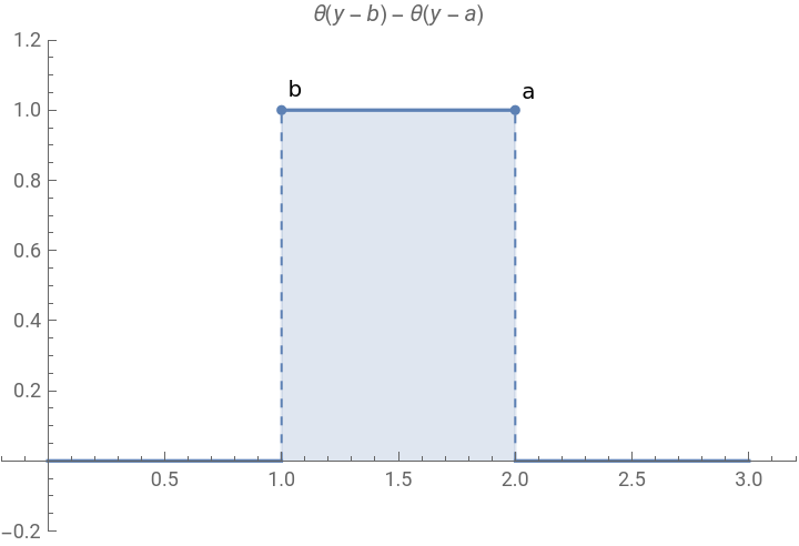
Given eigenvalues decaying as obtain expression for loss after t gradient descent steps using Laplace transform, compare against simulation.First construct Heavy function to convert b..a interval into 0..∞ Assuming decreasing g(x), will need b=g(∞), a=g(0), b<a
1
2
x
In[]:=
With[{bb=1,aa=2},points=ListPlot[{Labeled[{aa,1},"a"],Labeled[{bb,1},"b"]},FillingAxis,FillingStyleDashed];theta=HeavisideTheta[y-bb]-HeavisideTheta[y-aa];label=HoldForm[HeavisideTheta[y-b]-HeavisideTheta[y-a]]//TraditionalForm;plot=Plot[theta,{y,0,3},Filling->Axis,PlotRangePadding->.2,PlotLabellabel];Show[plot,points]]
Out[]=
Obtain f(t) using Laplace Transform
In[]:=
g[x_]=;gi=InverseFunction[g];a=g[0];b=g[∞];theta=HeavisideTheta[y-b]-HeavisideTheta[y-a];sol1=LaplaceTransform[D[gi[y],y]*y*theta,y,t]//FullSimplify
1
2
(1+x)

Out[]=
π
Erf[t
]2
t
Obtain f(t) using original definition
In[]:=
sol2=Integrate[g[x]Exp[-tg[x]],{x,0,∞}]
Out[]=
π
Erf[t
]2
t
In[]:=
Reduce[sol1==sol2]
Out[]=
True
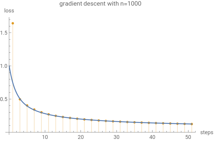
Obtain f(t) by running gradient descent on large n, compare against “infinite n” representations above
In[]:=
n=1000;(*dimensionoftheproblem*)maxStep=50;h=Table[1.,{i,1,n}];(*Hessianeigenvalues*)x0=ConstantArray[1.,{n}];(*startingpoint,producesaveragetrajectory*)xs=NestList[(#-h#)&,x0,maxStep/2];ys=Total[*h]&/@xs;steps=Range[Length[xs]]*2-1;(*correctformissingconstants*)discretePlot=ListPlot[Transpose[{steps,ys}],PlotLegends{"exact"},PlotStyle->ColorData[97][2],PlotRangeAll,Filling->Axis,AxesLabel{"steps","loss"},PlotLabel->StringForm["gradient descent with n=``",n]];continuousPlot=Plot[sol1,{t,0,maxStep+1},PlotRange->All,PlotLegends{"infinite-n"}];Show[discretePlot,continuousPlot,PlotRange->All]
2
i
2
#
Out[]=


Backward transformation from inverse Laplace transform
Backward transformation from inverse Laplace transform
In[]:=
Clear["Global`*"]
In[]:=
(*InverseLaplacegivesgi'ytheta,nowsolveforgi*)ilaplace=InverseLaplaceTransform,t,x
π
Erf[t
]2
t
Out[]=
1-HeavisideTheta[-1+x]
2
x
Manually get a,b by finding non-zero boundary, and get representation free of HeavysideTheta
In[]:=
Plot[ilaplace,{x,-2,2}]
Out[]=
In[]:=
{b,a}={0,1};(*g[0]=a,g[∞]=b,gi[a]=0*)theta=HeavisideTheta[x-b]-HeavisideTheta[x-a];Plotilaplace,theta,{x,-1,2},PlotStyle{Thick,Dashed}
1
2
x
Out[]=
In[]:=
F[x_]=Refine[ilaplace,{b<x<a}]
Out[]=
1
2
x
In[]:=
hi=Functiony,Evaluate@DSolveValuegi'[y]y==,gi[a]==0,gi[y],y
1
2
y
Out[]=
Functiony,
-1+
y
y