A self-avoiding walk (SAW) is a path through a lattice which never visits the same vertex twice. A multiway graph is a tree which starts in some initial position and connects each vertex to all possible next positions by a set of rules, generating expansive networks of states. For my project, I have explored SAWs through various grid lattices, generalizing to arbitrary dimensions and various surfaces including the torus, the Möbius strip, and the Klein bottle. I have generated multiway graphs representing all possible SAWs through these lattices, and provided a wide array of analysis on the resultant data.
N×N Lattices
N×N Lattices
Introduction
Introduction
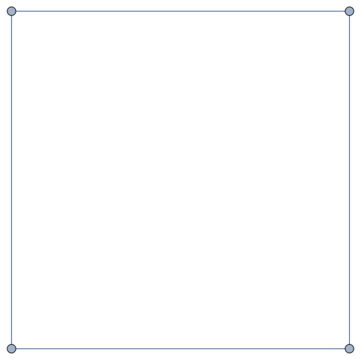
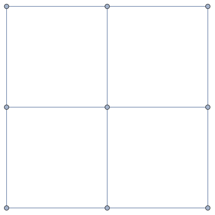
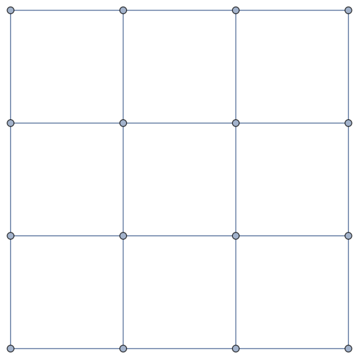
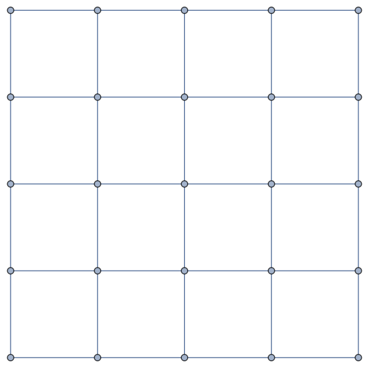
We begin with the simple case of an N×N square lattice. Examples of a 2×2, 3×3, 4×4, and 5×5 square lattice are given below
In[]:=
GridGraph[{#,#}]&/@Range[2,5]
Out[]=
,
,
,
Here is an example SAW through the 3×3 lattice. Green represents the starting vertex, blue the ending vertex, red the vertices visited by the walk, and black the vertices not visited by the walk
In[]:=
AnnotateshowWalk[{{1,8,7},{2,3,6},{0,4,5}}],VertexLabels->
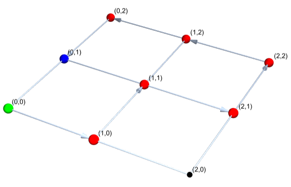
It will be useful at this point to define cyclic and Hamiltonian paths. A cyclic path, technically, is one where the ending vertex is the starting vertex. In our case, because the same vertex cannot be visited twice, we will consider a cyclic path to be one in which the ending vertex is adjacent to the initial. The above path is cyclic, by our definition. A Hamiltonian path is one which visits every vertex in the graph. The above graph is not Hamiltonian, because it omits vertex (2,0).
In this essay, I will consider a "lattice" to be the grid through which a walk progresses. A lattice can also be referred to as a "graph", though I will also use that term to refer to multiway systems. I consider "walk" and "path" to be synonyms, but "leaf" refers to a node on a multiway graph while "vertex" refers to a node on a lattice.
Lattice Walks and Multiway Graphs
Lattice Walks and Multiway Graphs
Representing lattice paths
Representing lattice paths
To begin coding, we need a way to represent lattices and paths through those lattices. One of the most versatile tools in the Wolfram Language is the list, and for our case it makes a lot of sense to represent lattices with 2-d arrays. Empty squares will be represented with 0s. So this 3x3 empty grid lattice
Out[]=
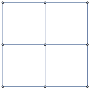
would be represented in our code by the array {{0,0,0},{0,0,0},{0,0,0}}. Now we need a way to show the path. In this case, we want a way to be able to trace the path back through time, so simply representing visited vertices with a 1 is out of the question. Instead, we will fill the board with successive integers, starting at 1. So the following path on a 3×3 lattice
Out[]=

Would be represented by the array {{1,2,3},{0,5,4},{0,6,0}}. This method is simple, generalizable, and allows me to use the vast repository of list manipulating functions available in Mathematica
Displaying a lattice
Displaying a lattice
I use a function I defined called showWalk for all of the visualizations in this essay. The main goal is to convert the grid representation of a walk that we use in our code into a graph representation, with appropriate color coding. The code for the function is explained below
We first need a function to convert a list of coordinates to a vertex index that we can use in a graph object. The function takes a coordinate like {3,1} and the size of the lattice
In[]:=
coordsToVertex[Nothing, n_] := Nothing;coordsToVertex[coords_List,n_Integer] := 1+Fold[n*#1+(#2-1)&, 0, coords]
The next helper function takes a grid representing a walk through a lattice and determines all of the edges, returning a list of the edges of a graph. Each edge is in the form {v1,v2} instead of v1v2 because lists are more versatile
In[]:=
walkEdges[graph_List] := Partition[coordsToVertex[Position[graph, #][[1]], Length[graph]]& /@ Range[Max@Flatten[graph]], 2, 1]
Our final helper function, getBasicGrid, just returns the basic grid graph of the lattice, with no directed edges to represent the path. It does do the color coding though, as that step is relatively simple
In[]:=
getBasicGrid[graph_List] := With[{length = Length[graph], max = Max[Flatten[graph]]}, GridGraph[Table[length, Depth[graph]-1], VertexStyle -> Flatten[Black, (*the following three lines are all color coloding*) coordsToVertex[#, length] -> Red & /@ Position[graph, n_/;1<n<max], coordsToVertex[Position[graph, 1][[1]], length] -> Green, coordsToVertex[Position[graph, max][[1]], length] -> Blue], (*this next line assigns the vertex sizes*) VertexSize -> Flatten[{0.05, coordsToVertex[#, length] -> 0.1 & /@ Position[graph,n_/;0<n]}] ]]
With this, we can construct our showWalk function, which just takes getBasicGrid and deletes and adds vertices to create directed edges corresponding to the actual path
In[]:=
showWalk[graph_] := With[{walk = walkEdges[graph], length = Length[graph]}, Graph3D[EdgeAdd[EdgeDelete[getBasicGrid[graph], UndirectedEdge @@@ walk], DirectedEdge @@@ walk ], VertexCoordinates -> Table[{Floor[(v-1)/length], Mod[v-1, length], 0}, {v, 1, Length@Flatten[graph]}]]]
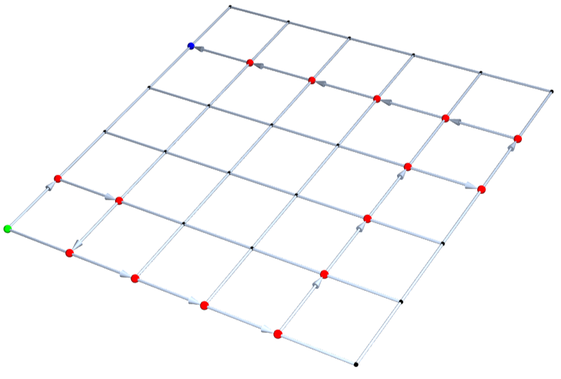
Here's an example of showWalk in action:
In[]:=
showWalk[{{1,2,0,0,17,0},{4,3,0,0,16,0},{5,0,0,0,15,0},{6,0,0,0,14,0},{7,8,9,10,13,0},{0,0,0,11,12,0}}]
Building basic functions
Building basic functions
We will want to create functions to create and manipulate lattice paths, so lets define a variable representing the starting position of a 2×2 path to use as an example
In[]:=
startingGraph={{1,0},{0,0}};
In[]:=
showWalk[startingGraph]
Out[]=

Our first goal is to create a function to find all the valid next positions, given a the state of an arbitrary SAW in the previously discussed list format. There are two things to consider:
◼
The next position must be within the graph (cond. 1)
◼
The next position cannot be an already-visited vertex (cond. 2)
The following code generates all possible next positions, given these two conditions
With this, we can generate a function, extendBoard, which returns a list of the possible next board states
This also works for larger lattices
Multiway graphs
Multiway graphs
A multiway graph is a graph showing all possible results from nestedly applying a fixed set of functions to a starting position. For our purposes, we can use multiway graphs to visualize all possible self-avoiding walks through a lattice, branching whenever there is more than one possible move.
Let's just have a function for generating starting graphs first
We can greate a multiway graph function which uses the resource function "Multiway System" to do the legwork for us
Here's the multiway graph representing all SAWs through a 2×2 lattice
How about a function to see the general shape of a larger system?
We can use this to visualize the multiway graph of all possible SAWs through a 4×4 lattice
Data Analysis: Terminal States
Data Analysis: Terminal States
Data extraction
Data extraction
We begin by getting our data in the form of variables
These variables represent multiway graphs, where each vertex is itself an array representing the state of an SAW at a particular moment. The data is visualized without the showWalk function, so that the general structure is more clear. threeData is drawn out below for reference
Let's just figure out the size of data we're working with
Here's a (not necessarily terminal) random example state from each of our datasets
Terminal leaves
Terminal leaves
Let's write a function to get just the terminal leaves of the graph. We define a terminal leaf to be any vertex which has no children- that is, one in which there are no remaining moves
What this code does is it run through the list of vertices in a multiway graph and selects those with 0 possible next moves, which are the terminal leaves
How many terminal states are there in each dataset?
Hamiltonian paths
Hamiltonian paths
As previously defined, a Hamiltonian path is one which passes through every vertex. In this case, a Hamiltonian path loosely conjures the idea of a "win"-- the path was able to fulfill every vertex without ever getting stuck. Let's figure out the portion of terminal states which are Hamiltonian for each of our datasets. Let us denote the frequency of terminal states which are Hamiltonian as h
The following code gets the number of Hamiltonian paths in the datasets
This data would be more useful if we found the frequency of Hamiltonian paths out of all finished paths- a.k.a h
It's obvious that the portion of graphs which are Hamiltonian drastically declines as the size of the lattice grows. By the 5x5 lattice, it is only about 2%. I think this comes from the fact that for larger lattices, there are simply more spaces to fill. Most of the non-Hamiltonian terminal states on an N×N lattice are also non-Hamiltonian on an (N+1)x(N+1) lattice, and those that aren't have some analogous non-Hamiltonian path, and there are tons more that arise from the increased freedom. The number of Hamiltonian paths, on the other hand, increases far more slowly.
A Hamiltonian path has 0 unvisited vertices. In the previous analysis, we considered the binary between 0 unvisited vertices and more than 0 unvisited vertices. However, we could just as easily consider the frequency of specific numbers of these vertices. For example, the below graph has three unfilled vertices
In general, we can plot as a histogram the number of graphs with x unvisited vertices
Terminal positions
Terminal positions
Where are the most common places in the grid for the walk to terminate? We can actually extract the positions of the terminal vertex from the terminal leaves of a dataset. Plotting a 3D histogram of the resultant coordinate lists gives some very nice graphs.
There are all sorts of interesting insights here. First of all, notice that the coordinate {1,1} is always empty, because as the starting position it is impossible for it to be the end state as well. going further, we see as a general trend that the corners (including the two squares adjacent to the starting square) seem to be by far the most common places for a path to terminate. This makes the most sense, as upon entering a corner vertex there can be at most 1 valid next position. Interestingly, the edges do not seem to be the next most common termination place. The following bar function allows me to generate bar charts formalizing this concept. The bar charts show the frequency of terminating a certain Manhattan distance from a corner (with the two vertices adjacent to the starting corner considered corners themselves, which a visual analysis of the data suggests is a valid approach), normalized for the number of edges with a certain Manhattan distance from the corners
The fact that the edges are less common as a terminal location than the center surprises me. I believe that this is because when the path is on an edge, it is usually running along the edge, and is likely to make it into a corner before terminating. The paths all come from a single point in the bottom left, so it's quite difficult to maneuver a path which is at an edge and is blocked in both of the two directions it can normally go from there. For this to occur, it basically has to go all the way to the other side, then backtrack, which is something that occurs in only a small portion of plots.
Data Analysis: Branch Creation Rate
Data Analysis: Branch Creation Rate
Introduction
Introduction
Up until now, the analysis we have done has considered only terminal states. We've only been interested in viewing walks in full, as opposed to taking the graph as a whole into account. In this section, I ask questions which can be answered without knowing the terminal states, such as: At what rate are new branches added? In what direction is the path typically traveling at a certain point? Because these questions don't require knowledge of the terminal states, we can consider them on lattices of arbitrary size.
Data extraction
Data extraction
We begin with the same data as earlier
But we can now consider boards of larger side lengths, allowing the graphs to be incomplete
We can get the vertex count of each of our datasets
Note that many of the later datasets seem to have almost exactly the same vertex counts. This will be explained shortly.
Creating the graphs
Creating the graphs
The rate of branch creation over time in the multiway graphs is a meaningful problem in the study of SAWs. It represents the average number of possible moves from the current position after a certain number of moves.
The following function creates an association between each of the lattice states with n 0s in the multiway graph and their corresponding number of next possible positions
We can then use that in this function which determines the average number of next possible moves for each layer down to a certain depth
Now let's get some nice list plots to represent the branch creation rate over time!
In depth analysis
In depth analysis
As previously explained, the first four plots represent the complete data of the entirety of the multiway system, while the last eight give data for just the first twelve moves on larger graphs. In fact, the graphs do seem to be following a neat, recognizable pattern. The branching rate begins at 2, because no matter the board size there are always 2 initial moves. In fact, there are also only 2 possible moves after this, because both of the first moves take the path to an edge, from which position there are two possible moves (except in the 2×2 case, where the path comes immediately to a corner). After this point, the branching speed seems to grow rapidly to a maximum, around 2.5 or 2.6. It can be proven trivially that this maximum number will always be less than 3, but will it approach 3 asymptotically as the lattice size is increased, or is it bounded by some smaller number, like 2.7 or 2.8?
Another interesting thing to note is the fact that all of the functions have a dip at 4. It's less obvious in the earlier graphs, but that's only because the ranges are different; there is still a definite dip of about 0.1 at 4. I think that this is because the paths with 4 vertices filled, a.k.a the third move, are the first which can "double back" on themselves. Before this point, there were no left moves or down moves. The third move has paths such as that shown below, where because the path has doubled back it can be restricted by vertices it has already passed through. This decreases the amount of possible moves, leading to the dip. The reason this does not continue is that the number of new paths into the middle rapidly becomes a more important factor than how many graphs are doubling back on themselves.
Finally, one other very interesting aspect of the plot is how repetitive it is. In fact, we can generally state that for an NxN lattice, the first N-1 values on the plot will be exactly the same as the first N-1 values for the (N+k)×(N+k) case, where k is a positive integer greater that or equal to one. For example, the first 5 points on the line plot for the 6×6 lattice are exactly the same as the first five points on the line plots for the 7×7 lattice, the 8×8 lattice, the 9×9 lattice, and so on. The reason for this is that up to a certain move number, the size of the lattice does not matter. If you have only gone 3 moves, than an 6×6 lattice is the same as a 7×7 lattice. The lattice size N only comes into play on the Nth move, therefore all of the data for m moves on a lattice (including the branching ratio data) will be identical for all lattices of size N>m.
The following code finds a random path of length 3 on a 6×6 lattice and shows that the corresponding path of a 7×7 lattice is functionally identical
This is also the reason why many of the datasets have similar vertex counts. twelveData and thirteenData have 61,715 and 61,717 vertices respectively, a difference of only two! The reason for this is because the number of lattice size doesn't matter until the move number "catches up" with it, and because we are only considering 12 moves, it is only in the last move that the data for the 12×12 and 13×13 lattices diverge, and even then only in two different states (those that go straight up or straight to the right). For those two paths only will there be a difference, namely that each of the two straight paths 12×12 board has only one possible moves at that point in time, while the respective paths on the 13x13 have 2 possible moves each, giving the observed difference of 2 vertices.
The following data first shows all the possible next moves after proceeding 12 squares vertically on a 12x12 or 13x13 lattice It can be seen that there is only one next move for the 12x12 lattice, and two for the 13x13.
Random SAWs
Random SAWs
Introduction
Introduction
Our previous analyses were severely limited by the size of the multiway graphs we could compute. We calculated every possible end state for the walks, which was very computationally expensive for large lattice sizes. Even with the branch creation rate analysis, our data was difficult to generate and we were bounded in how large our lattices could become while still returning useful information. In this section, we aim to find information about the terminal states of N×N grids with N ranging as far as we could want, allowing us to consider the limit as N goes to infinity. We will do this by generating our data statistically-- we will take a certain specified number of random self-avoiding walks and do our computation on that. This will allow us to consider very large graphs, while only doing computation on a much smaller sample size.
Random SAW generation
Random SAW generation
We need a function to generate a random self-avoiding walk. Thankfully, this is trivial with our previously defined functions.
Lets just have another function to get a certain number of these terminal states.
Pitfalls
Pitfalls
At first glance, this seems fantastic
The following code, theoretically, should give the portion of SAWs on an 8×8 grid which are Hamiltonian.
This is obviously ridiculous; there do exist Hamiltonian SAWs on an 8×8 lattice. An example is shown below. The reason we get this result is because the portion of SAWs on the 8×8 lattice which are Hamiltonian is so low that we are almost certain to get a sample of 1000 random walks which are all non-Hamiltonian, giving us an answer of 0. Of course, this normally doesn't present a problem, but it is a deficiency of the statistical method of analysis and should be considered.
This issue pales in comparison to another, far more pressing problem, which is that of bias. Consider the following multiway graph for an arbitrary system. If we were to do analysis on this graph, we would want to weight each of the ending states equally. However, as we can see, the probabilities of a random walk visiting each of these states vary. The path would be 3 times more likely to visit the leftmost vertex as the rightmost.
Importantly this is an unavoidable aspect of how a random walk works. A random walk only ever has local information about the probability of getting to the next states from the current position; that information is not enough to accurately and without bias simulate a random terminal state of a multiway function. For example, consider the following set of histograms that we developed earlier, representing the number of zeros in the terminal states of a 2×2, 3×3, 4×4, and 5×5 lattice respectively.
But now consider the following data, which is derived from a statistical sample of random walks.
The random walk data is highly distorted. We can't really retrieve the true distribution without normalizing for the number of path branches at each step, which would require us to know the structure of the multiway graph, which would eliminate any computational advantage we get from using statistical sampling.
◼
A "solution" to the statistical sampling problem
◼
The frequencies of the two end states are almost the same, which means that the algorithm is doing what we want. The problem is that it returns None 93% of the time. This will get worse exponentially as we increase the number of steps, making it totally useless for larger lattices, such as for this 5x5 lattice
◼
I could increase the number of iterations, but I would probably need hundreds of thousands, or even millions, before seeing a single actual solution. Thus, this method does not succeed in simplifying the computation time
All of this doesn't mean there is nothing interesting to be gleaned from random SAWs, but they cannot be used as a substitute for normal multiway graph method
Random SAW distance traversal
Random SAW distance traversal
Let's make a slight modification to how we've been thinking about SAWs, and start our path in the center of an arbitrarily large lattice. We will be approximating an infinite lattice. The question is this: on average, after n steps, how far is the "head" of the path from the origin position? Using random SAWs here lets us find how far we expect the walk to actually traverse, because we are now considering it in a more procedural sense.
The following function returns a sample of 1000 random SAWs in a theoretically infinite lattice (in practice I use a lattice just large enough for the path to never touch it)
Then I have a function which computes the mean euclidean distance from the center of the graph of the path "heads" of a set of SAWs
It is known that for a 2-d random walk (not necessarily self-avoiding), the average distance from the origin after N steps is Sqrt[N]. (MIT has a very good article on this subject). We can show that this is the case by creating a function to measure this ourselves. (the function is very simple, and can be run all the way up to 100 steps without much difficulty)
Now we can use our meanDistance function to compute the same graph for random SAWs
But the average distance from the origin in a SAW does not approach Sqrt[n]. It seems that for large n, Sqrt[n] < meanDistance[n] < n. This makes sense, because the self-avoiding walk can't move back towards the center once it has left; thus, one would expect it to move away from the center faster than the non-self-avoiding case.
Conclusion and References
Conclusion and References
Conclusion and Future Work
Conclusion and Future Work
In this essay, I have introduced a method for analyzing self-avoiding walks using multiway graphs. I have considered SAWs on arbitrary N×N grids, and determined their properties. I have generalized to consider higher dimensional lattices. I have considered statistical sampling of random SAWs, and examined their costs and benefits. I have further extended my functions to consider SAWs on various topological surfaces. I create numerous ways to represent these topological surfaces, embedding them in two and three dimensions. I have then discussed the concept of point-contractability, and structured a possible algorithm for determining whether or not a given walk is point-contractable.
I see many possibilities for future work in this area. I myself have begun developing functions to generalize my analyses to n-manifolds, that is, topological manifolds in n-dimensional space. The surfaces discussed above are by definition 2-manifolds, and the possibility of considering higher dimensional manifolds intrigues me. Another thing that I will definitely keep working on is the PCW algorithm. Time constraints disallowed me from writing a PCW detection algorithm for this essay, but it is a very conceptually interesting idea, and I'm intrigued to learn where it would go.
Acknowledgements
Acknowledgements
I would like to acknowledge the hard work on the part of Anne Marie, my mentor, who helped me on many occasions with troubleshooting and provided excellent feedback on various stages of my essay. I would also like to thank Rory, Eryn, and Megan for keeping the program running smoothly and enjoyably. I had a lot of fun!
References
References
◼
Random walks. (n.d.). https://www.mit.edu/~kardar/teaching/projects/chemotaxis(AndreaSchmidt)/random.htm
◼
This is an excellent discussion of random walks, including a proof that the root mean squared distance is the square root of the walk length.
◼
Wolfram Research, Inc. (n.d.). Möbius Strip -- from Wolfram MathWorld. https://mathworld.wolfram.com/MoebiusStrip.html
◼
This Wolfram MathWorld article is an excellent resource on the topology of Möbius strips, providing not only a parametrization for the surface, but also many other interesting properties like its perimeter and Gaussian curvature.
◼
Boy’s surface. (n.d.). https://mathcurve.com/surfaces.gb/boy/boy.shtml
◼
This is an post on the "Encyclopédie des Formes Mathématiques Remarquables" website which provides great information on the Kusner-Bryant parametrization, as well as good viualizations of Boy's Surface.
◼
Wikipedia contributors. (2023). Klein bottle. Wikipedia. https://en.wikipedia.org/wiki/Klein_bottle
◼
This Wikipedia article contains great information about the Klein bottle, including an entire section just on various parametrizations thereof.
CITE THIS NOTEBOOK
CITE THIS NOTEBOOK
Exploring self-avoiding walks with multiway systems
by Max Grunwald
Wolfram Community, STAFF PICKS, July 14, 2023
https://community.wolfram.com/groups/-/m/t/2964768
by Max Grunwald
Wolfram Community, STAFF PICKS, July 14, 2023
https://community.wolfram.com/groups/-/m/t/2964768