Cosine similarity is a common tool for comparing structured data, but it depends on fixed coordinate systems and does not naturally extend to relational representations such as graphs. Adjacency matrices provide a convenient matrix-based encoding of graphs, yet their comparison is sensitive to arbitrary vertex labeling. In this work, we examine graph similarity by sampling normalized matrix overlaps under random vertex relabelings, treating similarity as a distribution rather than a single value. We explore how these distributions behave across graph sizes and discuss how distances between distributions, such as the Kolmogorov–Smirnov statistic, may be used to compare graphs in a permutation-invariant manner.
0. Introduction
0. Introduction
Similarity is a foundational operation in modern machine learning. From word embeddings to attention mechanisms, many systems rely on cosine similarity or closely related inner products to compare representations and uncover structure in data. These methods are powerful precisely because they reduce comparison to simple linear algebra, enabling scalable computation in high-dimensional spaces.
However, cosine similarity implicitly assumes a fixed coordinate system: each dimension of a representation is assigned a consistent and meaningful role. When this assumption holds, as in learned embedding spaces, cosine similarity provides a robust notion of semantic alignment. When it does not, similarity becomes sensitive to arbitrary choices of indexing rather than underlying structure.
This limitation becomes especially pronounced in relational data. Graphs naturally represent relationships among entities, but their standard matrix representations depend on vertex labeling, which is often arbitrary. Two graphs may encode identical or near-identical relational structure while appearing dissimilar under coordinate-dependent comparisons. Exact graph isomorphism tests address identity but provide only a binary answer and fail to capture partial similarity in the presence of noise or perturbation.
In this research, we explore a probabilistic approach to graph similarity that relaxes strict label alignment. Instead of comparing adjacency matrices directly, we examine the distribution of Frobenius-normalized overlaps induced by random vertex relabelings. By treating similarity as a distribution rather than a single scalar, we obtain a statistical “fingerprint” that reflects how structural alignment behaves under arbitrary permutations.
This work is exploratory in nature. It does not aim to replace existing graph comparison methods such as graph kernels or learned embeddings, but rather to investigate whether permutation-induced overlap distributions can serve as a meaningful intermediate representation of structural similarity. Through empirical experiments on small graphs, we examine how these distributions behave across graph sizes and consider how they might be compared using nonparametric distance measures.
I. ‘Seeing’ Cosine Similarity
I. ‘Seeing’ Cosine Similarity
Cosine similarity became central to word2vec because it measures meaning by direction rather than magnitude. In word2vec, words are embedded as vectors in a high-dimensional space, and cosine similarity compares the angle between those vectors, capturing how similar their contexts are regardless of frequency. This makes semantic relationships emerge naturally: words that appear in similar contexts end up pointing in similar directions, enabling analogies, clustering, and semantic reasoning with simple linear geometry.
To those unfamiliar with cosine similarity, its the consequence of an operation in linear algebra known as a dot product. Geometrically, a dot product can capture the overlap in vectors, if they project in the same direction. Mathematically, it’s defined as follows:
Let ‘a’ and ‘b’ be vectors in a real space, then:
a
b
n
R
a
b
a
b
For visual learners, which is perfect, here’s are two random vectors created in three-dimensions. While easily visualized in two dimensions, this geometric interpretation extends to high-dimensional spaces, providing a robust framework for data comparison.

In[]:=
a.b
Out[]=
6.40758
Performing the dot product above shows the vectors graphed yield a value of 7.5. There’s a lot of ways you can interpret this, but here’s the angle which really captures its ‘similarity’:
In[]:=
VectorAngle[a,b]
Out[]=
0.230682
Do note that the operation returns this ϕ (from our equation above) in radians, which means the vectors are very closely aligned.
This should be a rough explanation as to why it’s important. In short, which I won’t go as much depth into, matrix multiplications are the core to modern deep learning (and most computer-intensive processes), and it can be interpreted as multiple cosine similarity operations over entries. This is the technology that empowers Transformers, which use multiple of these operations to identify underlying structure, or similarity between words across a sentence.
It’s a novel approach compared to the previously used and explored recurrence methodologies, which did fairly well to keep track of the past, but always evaluated a current state to some accumulation of the past. Instead, the transformer evaluated every word to every other word, giving each the opportunity to uncover semantic meaning.
VectorAngle
This should be a rough explanation as to why it’s important. In short, which I won’t go as much depth into, matrix multiplications are the core to modern deep learning (and most computer-intensive processes), and it can be interpreted as multiple cosine similarity operations over entries. This is the technology that empowers Transformers, which use multiple of these operations to identify underlying structure, or similarity between words across a sentence.
It’s a novel approach compared to the previously used and explored recurrence methodologies, which did fairly well to keep track of the past, but always evaluated a current state to some accumulation of the past. Instead, the transformer evaluated every word to every other word, giving each the opportunity to uncover semantic meaning.
II. Limitations of Cosine Similarity: The ‘Labeling’ Problem
II. Limitations of Cosine Similarity: The ‘Labeling’ Problem
Every representation comes with trade-offs, and cosine similarity is no exception. This section does not argue against its use. Instead, it highlights the assumptions under which cosine similarity operates and the kinds of structure it struggles to capture.
Cosine similarity compares objects by measuring the alignment between their vector representations. Implicit in this comparison is the assumption that each coordinate has a fixed and consistent meaning. When two vectors are compared, their indices are assumed to refer to the same features in the same order. Under this assumption, the dot product provides a meaningful measure of overlap.
This assumption holds in many embedding-based models. In word embeddings, for example, each dimension corresponds to a learned latent feature, and those dimensions are globally consistent across the embedding space. Rearranging the coordinates would destroy meaning, because the coordinate system itself is part of the representation.
However, not all data admits such a privileged indexing. In structural data, indices often function only as labels. Reordering those labels does not change the underlying structure, yet it can dramatically change the result of a dot product. Two representations may encode the same relationships while appearing dissimilar under a coordinate-dependent comparison.
In[]:=
MatrixForm[{c,d}]c.dN[VectorAngle[c,d]]
Out[]//MatrixForm=
1 | 2 | 3 | 4 |
3 | 1 | 4 | 2 |
Out[]=
25
Out[]=
0.585686
Above was an example. c is a vector {1, 2, 3, 4} and d is a vector {3, 1, 4, 2}. Geometry only encodes a meaning relative to the coordinate system, these live in different portions of space only because they’re assigned to the axes. The vector is not meaningful itself, its only when its indices correspond to some axis do they mean something.
If d is simply a permutation of c, are they different? By the axes, yes, they are different. But that’s only if we adhere to the axes, if we address it differently then they are different. A powerful representation would be one that doesn’t structurally change this radically.
If d is simply a permutation of c, are they different? By the axes, yes, they are different. But that’s only if we adhere to the axes, if we address it differently then they are different. A powerful representation would be one that doesn’t structurally change this radically.
This exposes a fundamental limitation of pairwise similarity: it is sensitive to how information is indexed rather than how it is structured. When representations describe relationships among many entities, meaning is not localized to individual coordinates but distributed across patterns of interaction.
We will return to this limitation experimentally later. For now, the key takeaway is that any comparison intended to capture structural similarity must be robust to arbitrary reindexing. It must recognize patterns independently of how they are stored. This requirement motivates a shift away from single vector comparisons toward representations and comparisons that emphasize relational structure rather than coordinate alignment.
We will return to this limitation experimentally later. For now, the key takeaway is that any comparison intended to capture structural similarity must be robust to arbitrary reindexing. It must recognize patterns independently of how they are stored. This requirement motivates a shift away from single vector comparisons toward representations and comparisons that emphasize relational structure rather than coordinate alignment.
III. Memory as a Relational Structure
III. Memory as a Relational Structure
We’ve talked about cosine similarity, but I want to shift to a different conversation: memory. Vector spaces optimize for linear operations, which is effective. But, the previous sections did outline the importance in relational invariances, which they can’t capture entirely. In short, they’re not a bad choice of expressing entities, but its missing stronger means of encoding relationships.
What does represent memory the most naturally? Graphs! Graphs express relationships far better than any other data structure: nodes can represent entities, edges represent connections of any kind, and weight quantifies those connections. It’s like travelling from Los Angeles to San Francisco, its doable, but that edge (the highways) have weight (the distance).
Word embeddings, like the previously mentioned word2vec, captures semantic similarity through vector direction, but they won’t represent relational facts. A knowledge graph would naturally do this, capturing relations effectively.
This is fairly a short section, mostly to give context and build a very natural progression toward the idea we’re building here.
IV. Isomorphism and Desire to Capture Uncertainty
IV. Isomorphism and Desire to Capture Uncertainty
The previous sections were written to build context. We know cosine similarity exists to capture ‘similarity’ in linear space, how it has limitations, and graphs being an alternative in constructing deeper relationships between entities.
Richard Assar of the Wolfram Institute has talked to me about graph neural networks (GNN), a method in deep learning that learns from connectivity. It aggregates information from neighborhoods to build node and graph embeddings, which can be similar to cosine-like similarity. But, invariance in node ordering is built into the GNN architecture and not imposed afterward.
The question I want to explore is if we can compare graphs in a way to capture their underlying relational semantics and remain computationally feasible. For the scope of the Winter School, I think this is a bit daunting, which warrants a sub-problem.
Stephen suggested an approach involving permutations of an adjacency matrix, a data structure used to encode nodal relationships. It’s binary, demonstrating the existence of an edge or not, instead of holding values.
In[]:=
g0MatrixForm[a0]
Out[]=
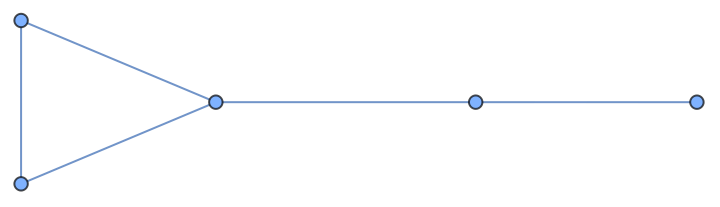
Out[]//MatrixForm=
0 | 1 | 0 | 0 | 1 |
1 | 0 | 0 | 0 | 1 |
0 | 0 | 0 | 1 | 0 |
0 | 0 | 1 | 0 | 1 |
1 | 1 | 0 | 1 | 0 |
As shown, a random graph with 5 vertices and 5 edges was constructed, along with its adjacency matrix. It’s difficult to read because the vertices aren’t labelled, but you can interpret it as each row and column capture if a vertex i is connected to a vertex j. The diagonal captures when i = j, with every other position capturing alternative combinations.
Let’s say you wanted to permute the graph as follows:
In[]:=
gPermutedMatrixForm[aPermuted]
Out[]=
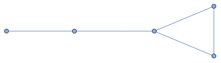
Out[]//MatrixForm=
0 | 0 | 0 | 1 | 1 |
0 | 0 | 1 | 0 | 1 |
0 | 1 | 0 | 0 | 1 |
1 | 0 | 0 | 0 | 0 |
1 | 1 | 1 | 0 | 0 |
Had the vectors been spanned across linear space, they would’ve been likely deemed as different. How do we know if they’re truly the same? We can verify they’re isomorphic.
In[]:=
{MatrixForm[a0],MatrixForm[aPermuted],IsomorphicGraphQ[g0,gPermuted]}
Out[]=
,
,True
0 | 1 | 0 | 0 | 1 |
1 | 0 | 0 | 0 | 1 |
0 | 0 | 0 | 1 | 0 |
0 | 0 | 1 | 0 | 1 |
1 | 1 | 0 | 1 | 0 |
0 | 0 | 0 | 1 | 1 |
0 | 0 | 1 | 0 | 1 |
0 | 1 | 0 | 0 | 1 |
1 | 0 | 0 | 0 | 0 |
1 | 1 | 1 | 0 | 0 |
While functions like provide a rigorous binary check for identity, they offer little insight when graphs are merely similar but not identical. In real-world biological or social networks, noise is inevitable.
This research introduces a probabilistic measure of graph similarity. By treating the set of all possible overlaps as a statistical distribution, we generate a continuous ‘fingerprint’ for each graph.
Using this, we can start to create a framework to take steps in quantifying partial similarity, so the graphs are not penalized for being completely non-identical.
IsomorphicGraphQ
This research introduces a probabilistic measure of graph similarity. By treating the set of all possible overlaps as a statistical distribution, we generate a continuous ‘fingerprint’ for each graph.
Using this, we can start to create a framework to take steps in quantifying partial similarity, so the graphs are not penalized for being completely non-identical.
V. Permutation-Induced Overlap
V. Permutation-Induced Overlap
To move beyond binary graph isomorphism, we require a scalar measure that captures degree of structural overlap. This section introduces such a measure by extending cosine similarity from vectors to adjacency matrices.
The dot product between vectors is a special case of a more general concept: an inner product. An inner product takes two objects and returns a scalar that measures how much they align, while obeying a small set of algebraic rules. These properties allow inner products to generalize beyond vectors to more structured objects.
The dot product between vectors is a special case of a more general concept: an inner product. An inner product takes two objects and returns a scalar that measures how much they align, while obeying a small set of algebraic rules. These properties allow inner products to generalize beyond vectors to more structured objects.
〈A,B〉
F
∑
i,j
A
ij
B
i
It’s similar to the vector dot product, but summing over all matrix entries instead of vector components. If you were to flatten the matrix into vectors, the Frobenius inner product is a standard dot product between those flattened representations. Relating to adjacency matrices, the quantity has a very simple interpretation. Because entries are binary, the Frobenius inner product counts a number of position where matrices have a 1, corresponding to a shared edge. Larger values indicate greater overlap.
Using what was shared above, the code to capture this product is shown below:
Using what was shared above, the code to capture this product is shown below:
In[]:=
overlapRaw[A_?MatrixQ,B_?MatrixQ]:=Total[Flatten[A*B]];overlapNorm[A_?MatrixQ,B_?MatrixQ]:=Module[{den=Norm[A,"Frobenius"] Norm[B,"Frobenius"]},If[den==0,0.,overlapRaw[A,B]/den]];
We also introduced another term: the Frobenius norm. This is normalizing the quantity and yielding a very cosine-like similarity metric for matrices.
overlap(A,B)
〈A,B〉
F
∥A∥B
∥
F
∥
F
∥A
∥
F
〈A,A〉
F
With the graphs we created before, let’s find their overlap with this function.
In[]:=
overlapRaw[a0,aPermuted]overlapNorm[a0,aPermuted]
Out[]=
4
Out[]=
2
5
How do you differentiate the two? is the Frobenius inner product, which does not have any sort of scale. It can grow large, but it’s not anchored or relative to anything. This is problematic. Imagine you have relatively small graphs and a few connections. You might count this as shared edges, but in small graphs, this is good.. As you see, we get the number 4, which makes us wonder how do you even interpret it.
But, performs a very similar operation to the cosine similarity we saw above. It tells us what fraction of the possible overlap do they achieve after correcting for how many edges each graph has. Taking the norm of each subject to these Frobenius conditions gives you a head count of the number of edges of the graph.
And as you see, between both graphs, and , it produces about 0.4. This means there isn’t a lot of overlap in the permutation. This sounds odd, so let’s create a new set of random graphs with labels.
overlapRaw
But,
overlapNorm
And as you see, between both graphs,
a0
aPermuted
In[]:=
Row[{g1,g2}]
Out[]=
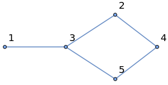
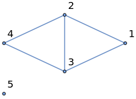
In[]:=
N[overlapNorm[a1,a2]]
Out[]=
0.6
We can see the two graphs might share some commonalities. For instance, 1 is connected to 4 in both. Same as 2 and 5.
And a final case before we transition to the next section, let’s try to compare a graph to itself and see how this looks. Cosine is 1 when its ϕ = 0, which geometrically means for vectors when two vectors overlap perfectly in space they’re a match. We’d want a similar metric to that, which is demonstrated below.
In[]:=
Row[{g1,g1}]
Out[]=
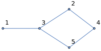
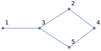
In[]:=
overlapNorm[a1,a1]
Out[]=
1
This definition captures overlap under a fixed vertex alignment. In the next section, we examine how this quantity behaves when vertex labels are treated as arbitrary, by sampling overlaps across random permutations.
VI. Overlap Distributions Under Random Relabelings
VI. Overlap Distributions Under Random Relabelings
With the concept introduced, we have a way to capture underlying structure. But, this is quite a weak concept to apply on graphs without knowing the kind of behavior it should warrant in larger settings.
One permutation is relatively meaningless, while many random permutations generate a distribution of overlaps that reflect structural similarity. The new question is that if a single overlap value isn’t conclusive enough, what is? That leads to the highlight of this section, distributions of overlaps across permutations.
Let’s return to the matrices of the previous section, g1 and g2. First, we need to construct a function to handle the permutation, which finds a permutation matrix P, such that:
Given matrix A and P, then, PA
T
P
A
permutation
permMat
We can repeat this across a few iterations and the permutations change, meaning the overlap changes. For smaller cases like this, there is a lot of repetition.
Let’s try to permute g1 by itself.
I was curious about when does it begin to take this shape since its very iteration dependent. For a graph of 5 vertices, we can shuffle every permutation if we wanted.
Had we continued the iterations, we would’ve sampled a larger portion of permutations to capture this pattern. But, our approach has captured this relatively nicely. In a case of 5 vertices/edges, this is possible given the smaller search space.
So, why not we try different sized graphs, starting from 3 to 10 and observe their histograms. We’ll approach a larger set of iterations to try and reach a distribution as close as the actual exhaustive one. Because we saw that comparing the same graph to itself isn’t capturing isomorphisms, we can permute over one of their adjacency matrices instead of comparing two random graphs of the same condition (since the permutation is essentially doing the same thing).
So, why not we try different sized graphs, starting from 3 to 10 and observe their histograms. We’ll approach a larger set of iterations to try and reach a distribution as close as the actual exhaustive one. Because we saw that comparing the same graph to itself isn’t capturing isomorphisms, we can permute over one of their adjacency matrices instead of comparing two random graphs of the same condition (since the permutation is essentially doing the same thing).
As the vertex count increases, the behavior shows they’re less sensitive to change. With the smaller counts, like 4, a single difference given the sizes of the graph reflect a vast structural difference. It’s like finding a typo in an essay vs in a short poem, the latter is more noticeable whereas the former can be less impactful as you read further. In other words, as the number of vertices grow, almost all random permutations produce negligible overlap, even when the underlying graph is unchanged.
What can we take away from this? Single overlaps are meaningless, they do show graph equivalence, but they don’t highlight beyond that. Distributions visualize these differences with an overlap metric, one that quantifies how similar are the relations they express.
Even in small cases like graphs of 3 and 4 where they do undergo permutations and reconstruct itself, this doesn’t tell us much. Geometrically, this builds very similar intuition to the cosine similarity: our adjacency matrix lives in an n x n space and a permutation continues to live in this space. Computing a sample fixes a representative in this space, comparing it to other representatives, which measures a cosine-like similarity in this space.
Even in small cases like graphs of 3 and 4 where they do undergo permutations and reconstruct itself, this doesn’t tell us much. Geometrically, this builds very similar intuition to the cosine similarity: our adjacency matrix lives in an n x n space and a permutation continues to live in this space. Computing a sample fixes a representative in this space, comparing it to other representatives, which measures a cosine-like similarity in this space.
VII. From Overlap Distributions to Graph Distance
VII. From Overlap Distributions to Graph Distance
Everything has been a natural progression, but where do we go from distributions? Our motivation to build the distributions was to represent graph similarity in a probabilistic manner rather than isomorphisms. The distributions above across various size graphs show it is possible to capture overlap, with smaller graphs being more sensitive to perturbations and larger graphs assuming a Gaussian-like shape.
The Kolmogorov-Smirnov (KS) distance answers the question: what is the largest vertical difference between two different cumulative distributions.
The Kolmogorov-Smirnov (KS) distance answers the question: what is the largest vertical difference between two different cumulative distributions.
Concluding Remarks
Concluding Remarks
Recap: Because the limited time offered in the Winter School, I wasn’t able to explore section VII in the detail of rigor I’d like to. But, I feel this notebook demonstrates an interesting experiment and sets the foundation for both further study in probabilistic interpretations of graphs and determining a graph distance corresponding to two graphs.
What we found was that cosine similarity fails under relabeling, which is handled poorly when the axes shift and therefore the positions change. Instead, we opted for graphs to represent relational data without the same structural constraint, apart from indices corresponding to entries in the adjacency matrix.
Permutations capture a distribution of overlap across relabelings, which I found interesting it takes a Gaussian-like shape. A Monte-Carlo approach taking a sample rather than exhausting the permutations handled smaller cases, where I’d argue 10 vertices is a small case, but I’m curious how this framework would extend to larger cases. I’d imagine in a future case, pruning rules would serve importance in preventing isomorphic permutations from being expanded.
Limitations: Before going into open questions, it might be important to acknowledge limitations of what I’ve currently done. Relying on Monte Carlo sampling is definitely not the best approach for larger factorials as argued. It’s also sensitive to graph density, where sparse and dense graphs might yield different overlap distributions despite equal vertex counts. And it’s also not a replacement for GNN embeddings or graph kernels, but its a complementary statistics view and a different perspective in the problem.
Open Questions and Future Directions: As for open questions the work here has brought, how do we actually compare distributions? I admit part of the fault came from having a very informal distribution, a set of values in a Table, which was compared unproven. Not to mention, treatment of larger cases as talked about is also on the table for interpretation.
Recently, I came across this concept of a ‘betweenness oracle’ in graph reconstruction, which differs from a distance oracle (or a tool to report the shortest path distance between pairs of nodes). I do wonder if this has a place in future work, given that a betweenness oracle is described to be used in reconstruction algorithms. If we could reconstruct a graph G to H through a guided-permutation, would the complexity be a measure to how distant they are?
Ultimately, the distributions are to serve and distinguish non-isomorphic but similar graphs. The tests were done on a set of fixed graphs, where their edges and vertex count were of size n. This also opens another question, how does this extend to uneven cases where two graphs might be slightly similar with vastly different sizes, e.g. a summary of a book reflects that very book, but it sure doesn’t have the same detail. This ties into concepts of unsupervised learning which find optimal compressions, and I do feel it might be interesting to explore operations like multiplying adjacency matrices by itself to capture paths of higher lengths than 1.
Personal Reflection: Despite the short time, I’m satisfied by the work I performed during the program. A lot of the difficulty came in identifying an idea to work toward. My intention of participating in the Winter School was to build more abstract, conceptual thinking which should serve as pedestal for future research I’d like to do in the field of machine learning.
Acknowledgments
Acknowledgments
I would like to thank mentors Eric James Parfitt and Richard Assar for their extensive contributions to the development of these ideas. Richard’s depth of expertise played a key role in shaping the direction of the research and in distilling the many ideas we discussed, while Eric provided invaluable support in helping me understand the Wolfram Language and in navigating the logistics of the Winter School. Most importantly, I cannot thank them enough for their patience and understanding regarding my schedule; their support went above and beyond.
I am also grateful to Stephen Wolfram for taking the time to discuss my interests and for helping provide the broader direction for this work. The Winter School has been an exceptionally insightful experience, and I extend my thanks to the administrators, lecturers, and staff for making it possible.
I am also grateful to Stephen Wolfram for taking the time to discuss my interests and for helping provide the broader direction for this work. The Winter School has been an exceptionally insightful experience, and I extend my thanks to the administrators, lecturers, and staff for making it possible.
Experimental Setup
Experimental Setup
Read here at your own discretion, it’s probably best to leave modules here, such that it’s not jumbled around the essay.
References
References
1
.T. Mikolov, K. Chen, G. Corrado, and J. Dean (2013), “Efficient Estimation of Word Representations in Vector Space,” arXiv preprint arXiv:1301.3781.
https://arxiv.org/abs/1301.3781
https://arxiv.org/abs/1301.3781
2
.T. Mikolov, I. Sutskever, K. Chen, G. Corrado, and J. Dean (2013), “Distributed Representations of Words and Phrases and their Compositionality,” Advances in Neural Information Processing Systems. https://proceedings.neurips.cc/paper_files/paper/2013/hash/9aa42b31882ec039965f3c4923ce901b-Abstract.html
3
.A. Vaswani, N. Shazeer, N. Parmar, J. Uszkoreit, L. Jones, A. N. Gomez, Ł. Kaiser, and I. Polosukhin (2017), “Attention Is All You Need,” Advances in Neural Information Processing Systems. https://papers.nips.cc/paper_files/paper/2017/hash/3f5ee243547dee91fbd053c1c4a845aa-Abstract.html
4
.Wolfram Research, Inc. (2020), “PermutationGraph,” Wolfram Function Repository.
https://resources.wolframcloud.com/FunctionRepository/resources/PermutationGraph/
https://resources.wolframcloud.com/FunctionRepository/resources/PermutationGraph/
5
.Wolfram Research, Inc. (2024), “ProbabilityPlot,” Wolfram Language & System Documentation Center.
https://reference.wolfram.com/language/ref/ProbabilityPlot.html
https://reference.wolfram.com/language/ref/ProbabilityPlot.html
CITE THIS NOTEBOOK
CITE THIS NOTEBOOK
A probabilistic view of graph similarity via random relabelings
by Vishakh Menon
Wolfram Community, STAFF PICKS, January 15, 2026
https://community.wolfram.com/groups/-/m/t/3607608
by Vishakh Menon
Wolfram Community, STAFF PICKS, January 15, 2026
https://community.wolfram.com/groups/-/m/t/3607608