Duffing Oscillator -- one of the simples and oldest systems in history of chaos theory. But it took 4 decades to realize that chaos dwells within such simplicity. It was first proposed by German engineer Georg Duffing in 1918, but only in 1961 Yoshisuke Ueda discovered chaos and strange attractor dubbed latter “Japanese attractor”. Chaos theory is very young, younger than Quantum Mechanics.
Duffing Oscillator is very simple to understand. It is just 3 more things added to harmonic oscillator: damping, drive, and simplest nonlinearity. It is a classical double-well system.
Duffing Oscillator can exhibit a strange attractor -- a pattern that a chaotic system settles into over time, showing how complex and unpredictable behavior can still follow an underlying order. It illustrates how systems can be both predictable in their overall shape but unpredictable in the details, helping us understand and study chaotic phenomena.
Duffing Oscillator can exhibit a strange attractor -- a pattern that a chaotic system settles into over time, showing how complex and unpredictable behavior can still follow an underlying order. It illustrates how systems can be both predictable in their overall shape but unpredictable in the details, helping us understand and study chaotic phenomena.
A Poincaré section is a snapshot of a complex system’s behavior taken at regular intervals. When applied to a chaotic system, it can reveal the underlying structure called a strange attractor, showing patterns within the chaos. This helps scientists understand and visualize the order hidden within seemingly random behavior.
From this example we know that for a periodically driven planar example, the Poincaré section can be obtained by sampling at regular time intervals. Sampling can be done using , with an action having with an enclosing around the call to .
In[]:=
ex=Block[{δ=0.15,γ=0.3},Reap[NDSolve[{x''[t]+δx'[t]-x[t]+x[t]^3γCos[t],x[0]0,x'[0]0,WhenEvent[Mod[t,2π]0,Sow[{x[t],x'[t]}]]},{},{t,0,100000},MaxSteps∞]]][[-1,1]];
The strange attractor for these parameter values can be visualized using :
In[]:=
ListPlot[ex,PlotRange{{-1.5,1.5},All},PlotStylePointSize[0],PlotTheme->"Detailed"]
Out[]=
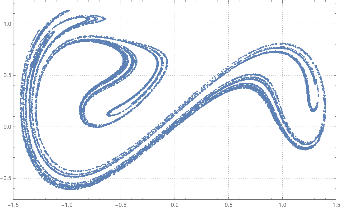
I wanted to extend this example by sampling Poincaré section not only at 2π, the period of driving force, but also at a multitude time stamps between 0 and 2π to see how different Poincaré sections look and smoothly animate thorough them. Lets define 50 such uniformly distributed events:
In[]:=
evs=Mod[t,2π]==#&/@(Range[0,2Pi-#,#]&@(2Pi/50));evs//LengthRandomSample[evs,3]
Out[]=
50
Out[]=
Mod[t,2π],Mod[t,2π],Mod[t,2π]
34π
25
4π
5
32π
25
The amazing efficient thing is that we need to run still just a single NDSolve because it can take a set of different WhenEvent:
In[]:=
data=Block[{δ=0.15,γ=0.3},Reap[NDSolve[{x''[t]+δx'[t]-x[t]+x[t]^3==γCos[t],x[0]==0,x'[0]==0,WhenEvent[Evaluate@evs,Sow[{x[t],x'[t]},Round[100Mod[t,2π]]]]},{},{t,0,100000},MaxSteps->∞]]];//AbsoluteTiming
Out[]=
{36.1123,Null}
We can see that sampling at different time leads to different patterns in the Poincaré sections:
In[]:=
ListPlot[data[[2]][[1;;50;;10]],PlotRange->{1.8{-1,1},1.3{-1,1}},PlotStyle->PointSize[0],PlotTheme->"Detailed"]
Out[]=
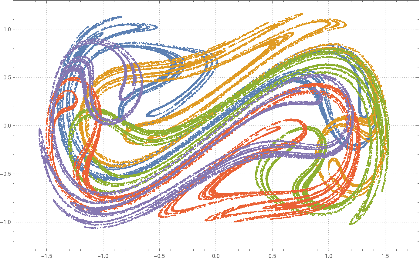
My plan is to animate through all Poincaré sections by smoothly chaining sampling time and keeping 13 different Poincaré sections on the screen at any given moment, but with fading away opacity, so closest to current time Poincaré sections are bright and the reset are forming a fading trace. I will redefine data format as follows:
In[]:=
newDAT=Join[#,#[[;;12]]]&@Most[data[[2]]];newDAT//Length
Out[]=
62
For the sake of artistic design and educational value I will define animated painting frame:
In[]:=
shift=30;blueFRAME=Table[{EdgeForm[Directive[Blue,Opacity[(11-n)/10],Thickness[.02]]],FaceForm[None],Rectangle[{-1.8+(n-1)/shift,-1.3+(n-1)/shift},{1.8-(n-1)/shift,1.3-(n-1)/shift}]},{n,10}];
and some key information:
In[]:=
ODE=TraditionalForm[Style[x''[t]+δx'[t]-x[t]+x[t]^3==γCos[t],30,Directive[White,Opacity[.7]]]];TTL1=TraditionalForm[Style["CHAOS AND STRANGE ATTRACTOR",30,Directive[White,Opacity[.5]]]];TTL2=TraditionalForm[Style["Poincaré Sections of Duffing Oscillator",30,Directive[White,Opacity[.7]]]];
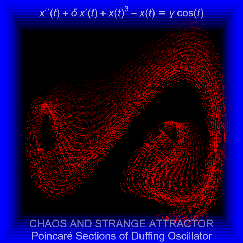
Here is how a single frame of animation looks:
In[]:=
ListPlot[newDAT[[1+13;;13+13]],PlotRange->{1.8{-1,1},1.3{-1,1}},AspectRatio->1,Axes->False,ImageSize->700,Background->Black,Prolog->blueFRAME,PlotStyle->Table[Directive[PointSize[0],Red,Opacity[k/16]],{k,15}],Epilog->{Inset[ODE,Scaled[{.5,.95}]],Inset[TTL1,Scaled[{.5,.08}]],Inset[TTL2,Scaled[{.5,.03}]]}]
Out[]=
The following builds all 50 frames:
frames=ParallelTable[ListPlot[newDAT[[1+s;;13+s]],PlotRange->{1.8{-1,1},1.3{-1,1}},AspectRatio->1,Axes->False,ImageSize->700,Background->Black,Prolog->blueFRAME,PlotStyle->Table[Directive[PointSize[0],Red,Opacity[k/16]],{k,15}],Epilog->{Inset[ODE,Scaled[{.5,.95}]],Inset[TTL1,Scaled[{.5,.08}]],Inset[TTL2,Scaled[{.5,.03}]]}],{s,0,49,1}];//AbsoluteTiming
Out[]=
{57.8814,Null}
and exports them into a .GIF file:
Export["Poincaré-Duffing.gif",frames,ImageSize->700,"DisplayDurations"->.07]
Out[]=
FIN-red-15-TTL-2L.gif
Alternatively you could create an .MP$ video:
In[]:=
Parallelize@FrameListVideo[frames,RasterSize->850,FrameRate->10]
CITE THIS NOTEBOOK
CITE THIS NOTEBOOK
Art from chaos & math: animated Poincaré sections of Duffing oscillator & its strange attractor
by Vitaliy Kaurov
Wolfram Community, STAFF PICKS, June 18, 2024
https://community.wolfram.com/groups/-/m/t/3195703
by Vitaliy Kaurov
Wolfram Community, STAFF PICKS, June 18, 2024
https://community.wolfram.com/groups/-/m/t/3195703