ORIGINAL ARTICLE: Fulvio Flamini, Marius Krumm, Lukas J. Fiderer, Thomas Müller, Hans J. Briegel (2023), Towards interpretable quantum machine learning via single-photon quantum walks, arXiv:2301.13669. DOI: https://doi.org/10.48550/arXiv.2301.13669
GITHUB: https://github.com/MariusKrumm/PhotonicsPS
GITHUB: https://github.com/MariusKrumm/PhotonicsPS
Article Abstract: Variational quantum algorithms represent a promising approach to quantum machine learning where classical neural networks are replaced by parametrized quantum circuits. However, both approaches suffer from a clear limitation, that is a lack of interpretability. Here, we present a variational method to quantize projective simulation (PS), a reinforcement learning model aimed at interpretable artificial intelligence. Decision making in PS is modeled as a random walk on a graph describing the agent’s memory. To implement the quantized model, we consider quantum walks of single photons in a lattice of tunable Mach-Zehnder interferometers trained via variational algorithms. Using an example from transfer learning, we show that the quantized PS model can exploit quantum interference to acquire capabilities beyond those of its classical counterpart. Finally, we discuss the role of quantum interference for training and tracing the decision making process, paving the way for realizations of interpretable quantum learning agents.
Licensed under the Apache License, Version 2.0 (the "License"); you may not use this file except in compliance with the License.
You may obtain a copy of the License at https://www.apache.org/licenses/LICENSE-2.0
Unless required by applicable law or agreed to in writing, software distributed under the License is distributed on an "AS IS" BASIS, WITHOUT WARRANTIES OR CONDITIONS OF ANY KIND, either express or implied.
See the License for the specific language governing permissions and limitations under the License.
Initialization
Initialization
Quantized Projective Simulation
Quantized Projective Simulation
Introduction — From classical to quantum projective simulation
Introduction — From classical to quantum projective simulation
Reinforcement Learning (RL) is a paradigm of machine learning that involves an agent interacting with an environment (see Fig.1a).The agent receives from the environment an input s ∈ S, called state or percept, and decides what action a ∈ A to take next. RL typically considers Markov decision problems, for which the agent's policy can be described by a conditional probability distribution π(a|s).The agent receives immediate feedback on its actions through a reward R; its goal is to find the policy that maximizes the long-term expected reward. In this post we focus on projective simulation (PS), a physically motivated RL model that has been applied to the study of collective behavior, robotics, automated design of quantum experiments and protocols, and quantum error correction.
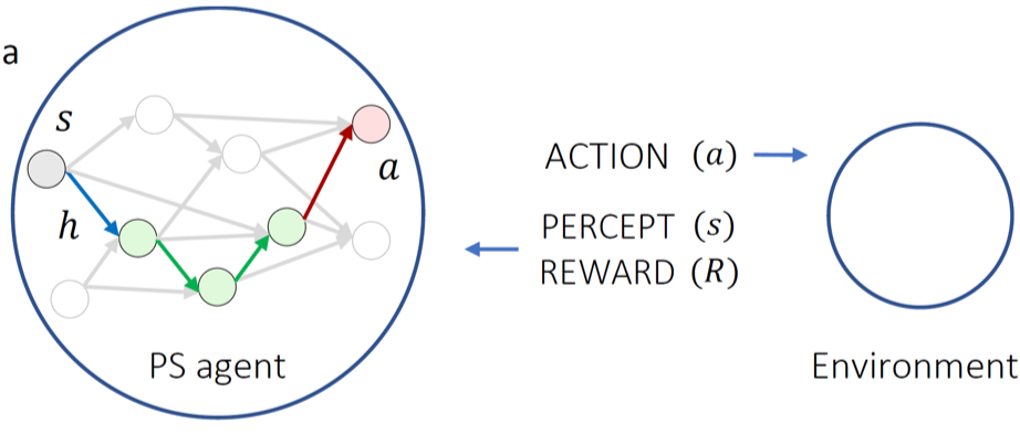
Figure 1a — When a PS agent receives a percept s from the environment, it initiates a random walk in the graph that describes its memory, until it hits a vertex representing an action a.
The performed action may be rewarded, leading to an update of the parameters (h-values) that control its decision making process.
The performed action may be rewarded, leading to an update of the parameters (h-values) that control its decision making process.
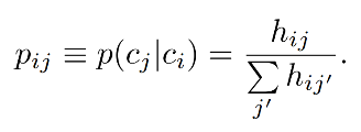
PS relies on a memory structure called episodic and compositional memory (ECM), described by a directed graph (see Fig.1a). The vertices of this graph, called clips, are associated with memories of the agent such as remembered percepts, actions or intermediate, more complex steps in the decision making process. This means that a clip carries semantic information. When the environment delivers a percept s, the corresponding clip is excited, and a random walk of a single excitation is initiated in its clip network, until the excitation hits an action clip a. This random walk in the ECM can be interpreted as a chain-of-thought that led to the decision. Each directed edge from clip to clip is associated with an unnormalized transition probability called h-value. The transition probability p(|) is computed by normalizing over all clips that can be reached from Learning occurs by changing the topology or the edge weights of the clip network, i.e. by tuning the h-values, which are initially set to 1. To this end, each edge with h-value is additionally equipped with a so-called glow factor , which contributes to the standard PS update rule:The role of the glow factor is to remember transitions ( → ) taken in past interactions with the environment, so that they are reinforced when a reward R is received. Further, γ ∈ [0, 1] is a forgetting factor: its main purpose is to gradually dampen previously learned transition probabilities, to let the agent adapt to changing environments. γ is also used as a soft cut-off to prevent the h-values to overflow. Each is updated as:where (0) = 0 and η ∈ [0, 1] is a discount factor for the actions taken further in the past. We refer to the literature on PS for a more detailed description and additional mechanisms, such as association and reflection.
c
i
c
j
h
ij
c
j
c
i
c
i
h
ij
g
ij

g
ij
c
i
c
j
g
ij

g
ij
Quantization of PS — Since decision making in PS is generated via a random walk of an excitation, it is possible to quantize it by giving learning agents access to a quantum walk in a quantum memory. Here we propose a quantum extension of PS that allows for a linear-optical implementation. Our guiding principle is to design a PS agent natively as a quantum walk of a physical excitation. To quantize PS, we need to quantize its main elements: the episodic memory, realized by the clip network, and the decision making process, described by the propagation of an excitation through the clip network. For an optical implementation, clips ∈ C (including percept clips, action clips and intermediate clips) then correspond to modes in an optical interferometer. For the quantization, we associate with each clip a pair of creation and annihilation operators of the corresponding (optical) mode, {, }. An excitation of memory clip at time is then described by the quantum state () |vac〉, where |vac〉 denotes the vacuum state, describing the inactive state of the agent’s memory. Here we use the Heisenberg picture where the operators carry the agent’s internal time dependence. Note that we index RL steps with t, while physical time within a step is denoted by . A decision-making process is initiated by the excitation of some clip at time . The evolution of the agent’s memory will be described by a unitary of the form
c
i
c
i
†
c
i
c
i
c
i
τ
0
†
c
i
τ
0
τ
k
c
i
τ
0

which relates the excitation operators of the clip network at different times. The Heisenberg time evolution of the ECM U(, ) is realized by the interferometric scattering matrix connecting the modes, which, in turn, is composed of a sequence of n intermediate transformations ,
τ
n
τ
0
ECM
U
k
U
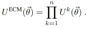
The are updated during the learning process via the set of parameters {θ} (see Fig.2b). To facilitate an optical implementation, here we consider ECMs described by a directed acyclic graph (DAG).
k
U

Table 1 — Links between the main elements of projective simulation (PS) and its proposed optical quantization.
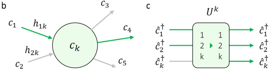
Figure 1bc — b) In classical PS, the vertices of the graph represent clips (). Directed edges are associated with transition probabilities that depend on the h-values.
c) In the quantized PS, clips are represented by mode operators describing a single excitation, while the connectivity is governed by mode-mixing transformations .
Each acts on the mode operators associated with the parent clips of (here , ), and its complex elements are the transition amplitudes that replace the classical probabilities of transitioning to .
All edges that contributed to the decision making process are in green.
c
k
c) In the quantized PS, clips are represented by mode operators
†
c
k
k
U
Each
k
U
c
k
c
1
c
2
c
k
All edges that contributed to the decision making process are in green.
Percept encoding — When the agent receives a classical percept at time , this leads to the excitation of a percept clip s. The quantum state of the memory is then described by () |vac〉. Subsequently, a quantum walk through the clip network starts.
τ
0
†
c
s
τ
0
Quantum walk in the ECM — To connect the random walk in the ECM to the quantum walk considered in this work, let’s take a look at the examples in Figs. 1 and 2. As shown in panel Fig. 1b, a clip effectively acts as a node that routes incoming edges from sets of clips to other clips in the next step of the random walk. In the quantum ECM sketched in Fig. 1c and Fig. 2b, this mechanism translates into the application of a transformation , which mixes creation operators of incoming clips with . A general clip-to-clip transition → is then modeled by transformations that mix subsets of creation operators, so that the stochastic nature of PS manifests itself at the level of quantum amplitudes. A crucial departure from classical PS is that clips are now visited in parallel (in superposition, see Fig.1 c), and all regions of the ECM that are reachable from a percept via a sequence of contribute to the decision making process. As a consequence, the probability to find an excitation in action clip a at time (described by the quantum state () | vac〉 when starting with an excitation of percept clip s at time (described by () |vac〉) is given by the modulus square of the corresponding transition amplitude
k
U
†
c
k
c
i
c
j
k
U
k
U
τ
n
†
c
a
τ
n
τ
0
†
c
s
τ
0

where |; 〉 = () |vac〉 are the time-dependent eigenstates of the number operators ()() corresponding to an excitation being present in clip at time . The above equation entails a quantum interference of all paths. While in classical PS the excitation has a well-defined trajectory in the ECM, now the excitation can be delocalized over all the allowed modes (i.e., the quantum amplitude is in general non-zero for more than one mode at the same time). This aspect bears an interesting potential for the learning model.
c
i
τ
k
†
c
i
τ
k
†
c
i
τ
k
c
i
τ
k
c
i
τ
k
Action decoding — The decision-making process ends when is applied and the output states are measured. When the excitation is detected in an output state associated with an action, this action is coupled out. In all other cases, the excitation can be (i) routed back to other regions of the reachable ECM; (ii) discarded, exciting again the same percept. In general, one can also associate multiple output states with a single action.
n
U
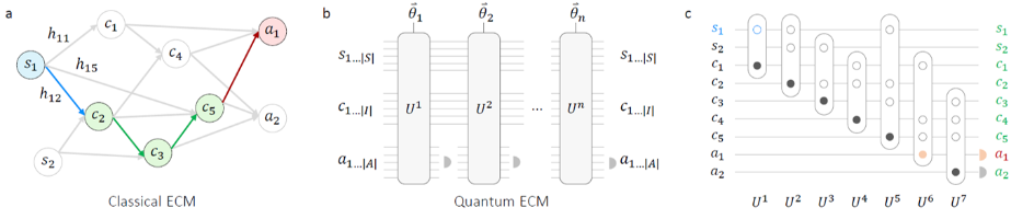
Figure 2 — a) In PS, decision making occurs via a classical random walk over a network of clips {, . . . , } that describes the agent’s episodic and compositional memory (ECM). When the agent receives a percept s (blue), an excitation triggers and performs a random walk over the network of intermediate clips {, . . . , } (green) until it hits one of the action clips {, . . . , } (red), which is immediately coupled out. b-c) In the proposed quantized PS, these random walks become quantum walks of single excitations through layers implementing the transformations , which mix sets of clips in a certain order. Here, clip-to-clip transition probabilities, classically described by the h-values, are replaced by transition amplitudes described by the matrix elements of . The evolution can be seen as hopping between eigenstates (of the modes) in the Hilbert space (empty disks: in/out modes; filled disks: output modes). Panel (c) reproduces the quantized evolution in the classical ECM in panel (a). Clips are now visited in superposition (green).
c
1
c
|C|
c
1
c
|I|
a
1
a
|A|
k
U
k
U
Training the quantum PS agent — To train the agent, we consider a variational approach based on a loss function ℒ that is inspired by classical PS and aims to reproduce its learning mechanism. ℒ depends on the probabilities {θ} to take action a given a percept s (that is, the policy) and the variational parameters {θ}. These probabilities can be estimated either numerically (by simulating the quantum walk) or experimentally (via multiple measurements with fixed input).
p
sa

The above framework (and much more) can be explored with this Mathematica package:
— Function 1 allows to study the structure of the proposed quantum ECM, starting from the directed acyclic graph (DAG) that describes the connectivity of the ECM. It can be used to test the learning model and to develop extensions.This function operates at an abstract level and does not presume an optical implementation. Functions 2-4 below can interact with its output by manipulating the transformations associated with each vertex of the DAG.
— Functions 2-4 allow to manipulate unitary transformations on a linear-optical circuit, with a focus on the canonical decompositions. These routines serve to instantiate the abstract representation of a quantum ECM, and allow to study arbitrary circuits as graphs.They handle the {θ}-parametrization in two formats, one for canonical architectures and one for arbitrary connectivities.
— Functions 5-6 enable the update based on the causal diamond for a 2-layer PS and multilayer PS. They make use of the graph representations given by Functions 1 and 4.
— Function 7 implements the update based on the Gram-Schmidt process.
— Function 7 implements the update based on the Gram-Schmidt process.
Below we initialize and visualize the structure of the ECM.
Visualizing the quantum episodic and compositional memory
Visualizing the quantum episodic and compositional memory
In the line with ★, choose between the Episodic and Compositional Memory (ECM) in the example of Fig. 2 (ECMfig2) or with a random, more complex, general, larger ECM (dag).
Below we initialize the quantum ECM. To do so, we choose a graph connectivity (randomly or predefined) and precompute quantities that help us manipulate and study any stochastic processes on this graph.
From left to right: (1) ECM in the example of Fig. 2; (2) same ECM with a layered structured that highlights which clip influences which; (3) same layered ECM color-coded according to the role of each node: percept clip (green), intermediate clip (black), action clip (red).
Here clips (nodes) are color-coded depending on the layer they belong to. Layers are constructed by looking at the causal dependencies in the underlying dag.
Here, nodes that are reachable from a given percept are colored in red. This snippet picks the percept with the subgraph withe the largest number of reachable clips.
Here we visualize the layered structures of the subgraphs of the ECM that are reachable from each percept clip.
Here we visualize all the relevant information and decision-making process related to a given percept (e.g., percept 1).
Quantum walk through the network of clips (each with its unitary transformation) starting from a given percept (e.g., percept 1).
Training the architecture
Training the architecture
Here we initialize the variables that we will use to train the architecture, in order to increase the probability to perform action a given percept s.
Here we train the architecture, in a toy model where we assume that at each step (inner loop) the environment issues a certain reward (outer loop).
Let’s now plot the probability to perform the chosen action a given percept s (see above), as a function of the number of steps of the training process.
Once the agent is trained, the unitary matrix that describes the decision making process in its ECM favors transitions from percept s to action a. In the plot below, this can be visible by looking at the black cells that correspond to successful (s,a) pairs. Here, columns represent percepts (s) and rows represent actions (a).
Towards interpretability — Partial traceability in the quantized projective simulation
Towards interpretability — Partial traceability in the quantized projective simulation
PS offers a viable framework towards designing interpretable learning agents, by allowing one to retrace the path taken between percepts and actions. We also know that this is no longer true in the quantum domain, since all paths contribute to the decision making process at once. The causal diamond (discussed further below in this notebook) allows us to make a first step toward the interpretability of quantum PS, by observing that a notion of partial trace can be recovered if one studies the likelihood that one photon (or more) would be measured in a given mode of the circuit (see Fig.5). This information can be retrieved by numerically simulating the single-photon quantum walk, since all phase settings are known. This possibility still holds for multi-photon quantum walks despite the hardness of the computation, which makes it practically feasible only for a small number of photons.
Figure 5 — Partial traceability in the decision making process of quantum PS agents. a-b) Two quantum walks,associated with as many 2-layer ECMs,are numerically simulated with a square optical architecture. Each panel shows the probability P to measure a photon in one of the output modes before training.Each column (label: Layers) displays the squared column (for a fixed percept) of the unitary matrix obtained by adding a new layer of optical elements,from left (input layer) to right (full circuit). The rightmost column of each plot corresponds to the output probabilities of a quantum walk over the full ECM. c-d) Same analysis after training with the causal diamond. Panels (c) and (d) correspond to the evolutions in panels (a) and (b),respectively.We observe that a notion of partial trace emerges inside the circuit, which can be leveraged to study interpretability in quantum learning agents.
Let’s now train the architecture using the causal diamond (described in the section below), tracking the likelihood that - if measured - a photon would be found in any of the intermediate optical modes in the circuit.
Initializing the parametrized circuit that will be used to simulate the training
Initializing all quantities that will be used to simulate the training
Training the architecture with multiple (s,a) pairs, while monitoring the scattering probabilities within the interferometers (i.e., not only at the output)
Here we plot the scattering probabilities for different (s,a) pairs, as described in more detail in Fig. 5 above.
Here we plot the scattering probability for different (s,a) pairs. The fact that the same combination of phase settings can optimize this many pairs is non-trivial.
Variational approaches to train the architecture
Variational approaches to train the architecture
Based on causal diamonds
Based on causal diamonds
Square architecture
Square architecture
Here we initialize the parametrized linear-optical interferometer
Here we update the phase settings of the interferometer using the variational algorithm based on the causal diamond. We assume that there are multiple (s,a) pairs that are rewarded.
Here we plot the learning curves resulting from the training process, for all rewarded (s,a) pairs.
Here we visualize an example of causal diamond in the graph describing a linear-optical interferometer of size DIM
Here we visualize an example of multiple causal diamonds (different colors) in the graph describing a linear-optical interferometer of size DIM
Based on the Gram-Schmidt orthonormalization process
Based on the Gram-Schmidt orthonormalization process
Optimization
Optimization
Here we test how this update mechanism performs when there are multiple rewarded (s, a) pairs.
We will suppose there are five rewarded (s,a) pairs: (1,1),(1,2),(2,1),(2,2) and one additional pair chosen by the user (updatedIN,updatedOUT), which are updated with different frequencies.
We will suppose there are five rewarded (s,a) pairs: (1,1),(1,2),(2,1),(2,2) and one additional pair chosen by the user (updatedIN,updatedOUT), which are updated with different frequencies.
CITE THIS NOTEBOOK
CITE THIS NOTEBOOK
Towards interpretable quantum machine learning via single-photon quantum walks
by Fulvio Flamini, Marius Krumm, Lukas J. Fiderer, Thomas Müller, Hans J. Briegel
Wolfram Community, STAFF PICKS, November 19, 2023
https://community.wolfram.com/groups/-/m/t/3067403
by Fulvio Flamini, Marius Krumm, Lukas J. Fiderer, Thomas Müller, Hans J. Briegel
Wolfram Community, STAFF PICKS, November 19, 2023
https://community.wolfram.com/groups/-/m/t/3067403