Bi-radial Matrix
Bi-Radial Matrix: Scaling Mechanism
By Russell Kramer
By Russell Kramer
Biradial Manipulate
Biradial Manipulate
Begin Package
Begin Package
BeginPackage["BiRadialMatrix`", {"GeneralUtilities`"}]
Needs[# <> "`", FileNameJoin[DirectoryName[$InputFileName], # <> ".wl" ]]& /@ { "BiradialPlot"}
Usage Statements
Usage Statements
SetUsage[BiradialManipulate, "BiradialManipulate[]"]
Begin Private
Begin Private
Begin["`Private`"] (* Begin Private Context *)
Manipulate
Manipulate
BiradialManipulate[] := DynamicModule[ pha = 0, phb = 0, phaseSync = False, phaseInverse = False, showLabels = False, mirrorRayNumbering = False , Manipulate[ BiradialPlot`makeBRMPlot[ d, ra, rb, pha, phb, rule, plotRange, "showPointLabels" -> showLabels, "lineThickness" -> thk, "nodeDiam" -> nodeDiam, "imgWth" -> width, "lineColor" -> lineColor, "pointColor" -> pointColor, "mirrorRayNumbering" -> mirrorRayNumbering ], {rule, "rays", "Field Structure"}, "nodes" -> "Nodes", "rays" -> " Rays ", "attract" -> " Attract ", "repel" -> " Repel ", "hyperbola" -> " Hyperbola " , {{d, 4, Style["D", 14]}, 1, 6, 1}, {{ra, 24, Style[Subscript["R", "a"], 14]}, 4, 60, 1}, {{rb, 24, Style[Subscript["R", "b"], 14]}, 4, 60, 1}, Item[Grid[ Style[Subscript["ϕ", "a"], 14], Dynamic[Manipulator[ Dynamic[pha, (pha = #; If[phaseSync, phb = ra / rb If[phaseInverse, -pha, pha]]) &], {N[-π / ra], N[π / ra]} ]] , Style[Subscript["ϕ", "b"], 14], Dynamic[Manipulator[ Dynamic[phb, (phb = #; If[phaseSync, pha = rb / ra If[phaseInverse, -phb, phb]]) &], {N[-π / rb], N[π / rb]} ]] ], Alignment -> Right], Item[Grid[ "Phase Synch", Checkbox[Dynamic[phaseSync]], "Inverse", Checkbox[Dynamic[phaseInverse]] , "Show Labels", Checkbox[Dynamic[showLabels]], "Mirror", Checkbox[Dynamic[mirrorRayNumbering]] ], Alignment -> Center], {{thk, 0.002, "Line Thickness"}, 0.001, 0.01, 0.001}, {{nodeDiam, 0.01, "Node Diameter"}, 0.005, 0.02, 0.001}, {{lineColor, Purple, "Line Color"}, ColorSlider}, {{pointColor, Black, "Point Color"}, ColorSlider}, {{plotRange, 6, "Plot Range"}, 2, 12, 1}, {{width, 400, "Image Size"}, 400, 800, 100} ], SaveDefinitions -> True(* , SynchronousInitialization -> False *) ]
Package footer
Package footer
End[] (* End Private Context *)EndPackage[]
The Bi-radial Scaling Mechanism
The Bi-radial Scaling Mechanism
There are numerous geometric properties of the bi-radial matrix. In the previous two articles a direct geometric correspondence with gravitation and magnetism was indicated. As well a direct geometric analogy to time and space was developed corresponding to established geometric properties of time and space. From here it is possible to describe these field structures directly in terms of space and time. It is generally recognized that with respect to force fields the greater the spacing between the field lines the weaker the force in that region. Conversely the closer the spacing between the field lines the stronger the force in that region. It is also known that the forces on the atomic and sub atomic scale are very strong and extend over very minute distances or ranges. In contrast gravity is a very weak force exerting itself over vast distances. Is there a fundamental mechanism within the bi-radial matrix which corresponds to this transition between the microscopic and macroscopic scale with respect to the fundamental forces?
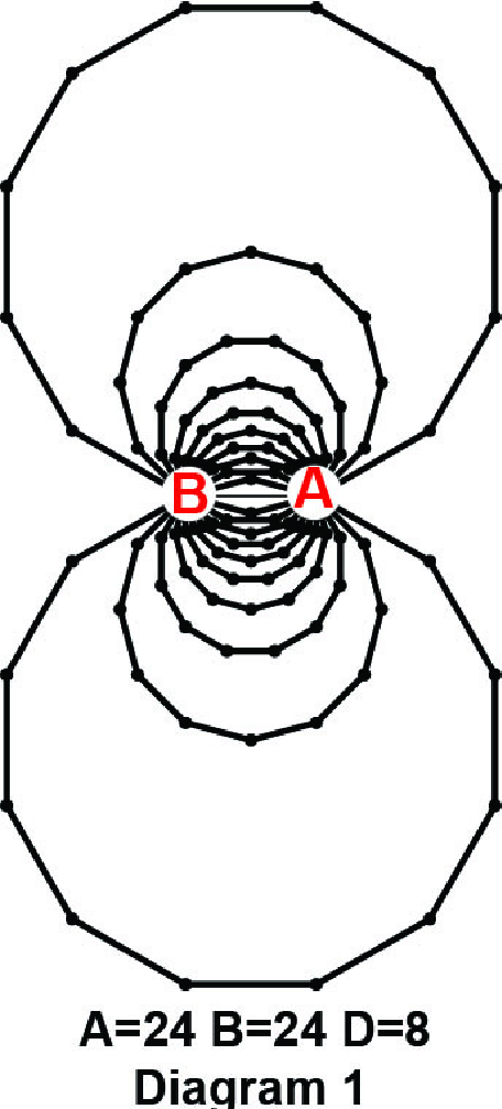
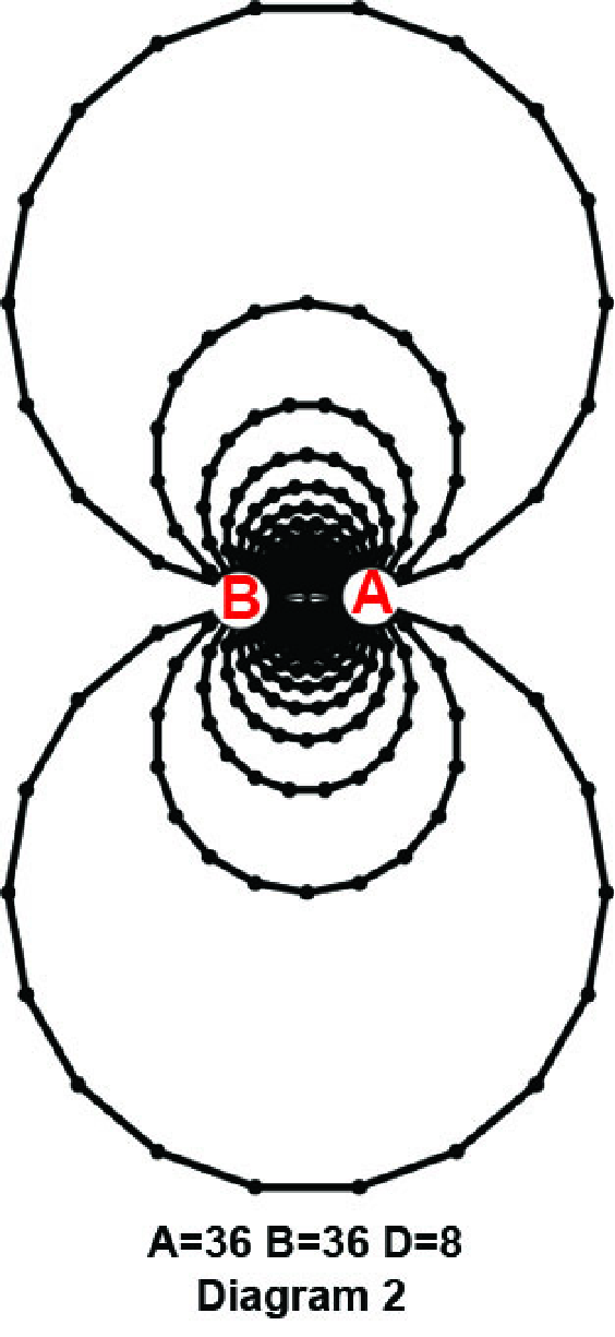
There are two techniques to alter the spacing of the field lines in the bi-radial matrix. This relates to the length of the D segment and the number of rays from each pole A and B. Recall the number of rays from pole A and B corresponds to mass and the gravitational field intensity “I”. Let us start with diagram 1 where the number of rays from each pole is 24 and the length of the D segment is 8 units. One way to decrease the distance between the force field lines is to increase the number of rays from each pole while leaving the distance unchanged. In diagram 2 the rays from poles A and B are increased to 36 with the distance remaining 8 units. We can casually observe a general decrease in the spacing of the force field lines indicating a stronger force between the two masses. Since the number of rays corresponds to mass this would be expected. This relates to the field intensity “ I”. The calculations for “I” are the subject of a future article.
There are two techniques to alter the spacing of the field lines in the bi-radial matrix. This relates to the length of the D segment and the number of rays from each pole A and B. Recall the number of rays from pole A and B corresponds to mass and the gravitational field intensity “I”. Let us start with diagram 1 where the number of rays from each pole is 24 and the length of the D segment is 8 units. One way to decrease the distance between the force field lines is to increase the number of rays from each pole while leaving the distance unchanged. In diagram 2 the rays from poles A and B are increased to 36 with the distance remaining 8 units. We can casually observe a general decrease in the spacing of the force field lines indicating a stronger force between the two masses. Since the number of rays corresponds to mass this would be expected. This relates to the field intensity “ I”. The calculations for “I” are the subject of a future article.
The other method to decrease the spacing of the force field lines is to decrease the length of the D segment while leaving the ray count unchanged. In diagram 3 the ray count from poles A and B=24 as in diagram 1 and the distance between the poles is reduced to 4 units, half the initial value of 8 units in diagram 1. Compared to diagram 1 we can casually observe the spacing of the field lines decreases towards the central region and rapidly increases. This again relates to the field intensity “I” which was referred to in part one of this series. Now there is an outer limit to where the rays intersect where there are no longer any intersection nodes and thus no field lines. This outer limit is referred to as the “range” of any given bi-radial matrix.These preliminary studies here are leading up to deriving formulas to calculate the range and field intensity. Now this entire process can be worked in reverse.
1) Increasing the ray and count decreasing the distance from each pole decreases the spacing of the force field lines
2) Increasing the distance between the poles and decreasing the ray count from each pole tends to increase the spacing of the force field lines.
1) Increasing the ray and count decreasing the distance from each pole decreases the spacing of the force field lines
2) Increasing the distance between the poles and decreasing the ray count from each pole tends to increase the spacing of the force field lines.
Visualizing the bi-radial Scaling Mechanism
Visualizing the bi-radial Scaling Mechanism
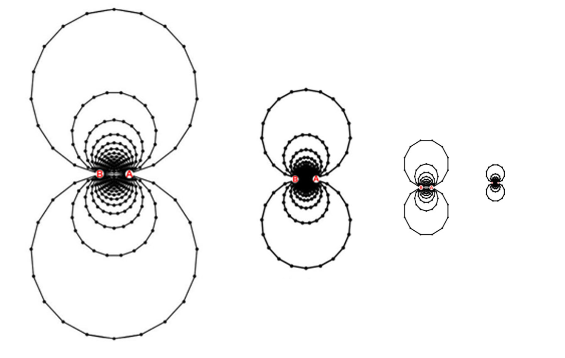
Now in diagrams 4A-4G we have a series of bi-radial matrices where in each successive one the D segment is halved in length while the number of rays from each pole remains the same. We can casually observe that both the distance between the force field lines decreases and the range of the field decreases. Were this process to continue to the atomic scale the resulting field lines would be spaced extremely close together with an extremely short range corresponding to a force field of enormous strength exerting itself over a very minute distance.This is consistent with the atomic and subatomic forces in general. In this analogy as indicated above decreasing the ray count (corresponding to smaller mass) increases the distance between the field lines which would seem to run counter to the forces on the microscopic scale. Yet at the same time the distances involved are so minute they supercede the ray count from each pole. Now the issue of defining a more detailed atomic force field structure requires a broader generalization of the bi-radial matrix where the number of poles is greater than two.This relates to the many body problem and will be dealt with in future articles.
Macroscopic Scale
Macroscopic Scale
To represent the bi-radial scaling mechanism on the macroscopic scale the number of rays from each pole A and B by strict analogy would need to be enormous. There is a way to use a lower sampling rate of rays and convey the essential information. This requires using the bi-radial equivalency principle. This can be illustrated using the bi-radial coordinate system. For general calculations we can regard the length of the D segment as unit measure. This could end up representing an astronomical unit or a Plank unit or anything in between; this relating to the bi-radial scaling mechanism.
In diagram 5A the number of rays from each pole A and B is 18. The set of nodes who’s coordinates satisfies the equation A=B fall along a vertical axis converging on the D segment such that the ratio of segments d1 and d2 are in the same ratio as A and B: 1/1. In diagram 5B the number of rays from each pole is 36. The set of nodes who’s coordinates satisfies the equation A=B also fall along the vertical axis converging on the D segment such that the ratios of d1 and d2 are in the same ratio as A and B: 1/1. The difference is that is diagram 5B there is a higher sampling rate of nodes along the vertical axis V and the nodes who’s coordinates are {1,1} converge closer to the D segment.
In diagram 5A the number of rays from each pole A and B is 18. The set of nodes who’s coordinates satisfies the equation A=B fall along a vertical axis converging on the D segment such that the ratio of segments d1 and d2 are in the same ratio as A and B: 1/1. In diagram 5B the number of rays from each pole is 36. The set of nodes who’s coordinates satisfies the equation A=B also fall along the vertical axis converging on the D segment such that the ratios of d1 and d2 are in the same ratio as A and B: 1/1. The difference is that is diagram 5B there is a higher sampling rate of nodes along the vertical axis V and the nodes who’s coordinates are {1,1} converge closer to the D segment.
In diagram 6A the number of rays from pole A is 36 and the number of rays from pole B is 18. The set of nodes defined by the equation A=B fall along the curve which converges with the D segment such that the ratio
d1/d2≈36/18. In diagram 6B the number of rays from pole A is 72 and the number of rays from pole B is 36-the same ratio as in diagram 6A. The set of nodes defined by the equation A=B also fall along the curve
which converges with the D segment such that the ratio d1/d2≈72/36. Thus both sets of nodes in diagram 6A and 6B fall along the same path. So we can thus define the bi-radial equivalency principle:
Bi-Radial Equivalency Principle
In any bi-radial matrix where the ratio of rays from each pole is the same and the distance D remains the same the set of nodes defined by
any given bi-radial equation will fall along the same path.
This applies to vertical axis, various curves along with the attraction and repulsion lines of force as well. This indicates that it is possible to define the plot of any bi-radial equation to varying degrees of accuracy
and approximation as needed. Now I refer to this as a principle because there is likely a formal mathematical proof which would take this from “principle” to established fact. The geometry here is somewhat advanced
and I’d welcome anyone who thinks they can formally prove the bi-radial equivalency principle to take a crack at it. Yes there are many areas of expertise that can be brought to bear here.
Now returning to the bi-radial scaling mechanism with respect to the macroscopic scale to diagram the macroscopic models a slightly different approach is in order. As the distance between objects on this scale
can be in the hundreds of thousands, millions, billions even trillions of miles diagramming this to scale is not feasible. We can for example establish a general tendency regarding the range of a bi-radial matrix as
the distance between poles A and B increases while the number of rays from each pole remains the same. Diagrams 7A-7F show a series of bi-radial matrices where the number of underlying rays from each pole
remains const ant at 24 and the distance doubles. This results in a broader increase in the range of the force fields. Note that some of the outer field lines in diagrams 7D-7F are arbitrarily cut off and the field structure
should be extending much further than indicated. We’re addressing this issue with respect to the programming code presently.
Diagram 7E Diagram 7F
Diagram 9C
Summary
Summary
The bi-radial equivalency principle was introduced to show how the bi-radial matrix can be used for calculations to varying degrees of accuracy. The bi-radial scaling mechanism was introduced revealing a detailed process by which the range and field density of the attraction lines can be scaled from microscopic to macroscopic by varying the distance D between the poles and varying the sampling rate of the rays from each pole. Within this singular structure based on a few simple parameters we have been able to explain how gravitation relates to forces on the microscopic scale from a structural standpoint. There is another generalization of the bi-radial matrix where the number of poles is greater than two(2). This is necessary for precisely modeling atomic structure because the inverse square laws do not always apply on this scale and more complex symmetry is necessary to model forces on this scale.
Now there is an enormous amount of work ahead. The purpose of these introductory articles is to demonstrate that this a very promising avenue of research. There are additional parameters to the bi-radial matrix. These include the absolute and relative phase relations which deal with rotation of the poles A and B and reveal the dynamic properties of the bi-radial matrix. There are field intensity equations and other basic properties of the bi-radial matrix and of course the range equations relating to the scaling mechanism. There are the inevitable comparisons to actual experimental and observational phenomenon and relating this work to current developments in quantum gravity. There are additional field structures embedded in the bi-radial matrix revealing the harmonic structure of space time on the most fundamental level.
Now there is an enormous amount of work ahead. The purpose of these introductory articles is to demonstrate that this a very promising avenue of research. There are additional parameters to the bi-radial matrix. These include the absolute and relative phase relations which deal with rotation of the poles A and B and reveal the dynamic properties of the bi-radial matrix. There are field intensity equations and other basic properties of the bi-radial matrix and of course the range equations relating to the scaling mechanism. There are the inevitable comparisons to actual experimental and observational phenomenon and relating this work to current developments in quantum gravity. There are additional field structures embedded in the bi-radial matrix revealing the harmonic structure of space time on the most fundamental level.
Afterthought
Afterthought
When going through my previous studies of the bi-radial matrix I encountered these large scale hand drawn (with straight edge) and written pieces relating to its internal structure. The diagram is based on a special case bi-radial matrix where the number of rays from each pole is 36. These go back a ways. If you can zoom in you will see I assigned variables to the interior angles and line segments along the rays. There are lot’s of associated trig equations on the other page. I need to review and double check these and redo the diagrams in Mathematica and use the classroom assistant to re-enter the equations in due time. In these studies the emphasis is on both the fundamental mechanisms and physical interpretation of the varied structures and components. There are formulas for the areas of the trapezoids such as shown in diagrams 5A-6B for instance. As a case in point it would be prudent to show how these trapezoids relate to the structure of attraction lines first. Otherwise we have an neat looking equation without a detailed physical interpretation. Further development of the bi-radial matrix continues in future articles.
Biradial Plot Functions
Biradial Plot Functions
Begin Package
Begin Package
Usage Statements
Usage Statements
Begin Private
Begin Private
makeBRMPlot
makeBRMPlot
Inner Functions
Inner Functions
Package footer
Package footer
Vector Geometric Functions
Vector Geometric Functions
Begin Package
Begin Package
Usage Statements
Usage Statements
Begin Private
Begin Private
Vector Geometric Functions
Vector Geometric Functions
Package footer
Package footer