Bragg peak aberration functions: X-ray powder diffraction in education
by Robert Dinnebier
This is the third part of three-part series for this work.
First part: https://community.wolfram.com/groups/-/m/t/2408912
Second part: https://community.wolfram.com/groups/-/m/t/2409355
by Robert Dinnebier
This is the third part of three-part series for this work.
First part: https://community.wolfram.com/groups/-/m/t/2408912
Second part: https://community.wolfram.com/groups/-/m/t/2409355
ABSTRACT: A collection of scholarly scripts dealing with the mathematics and physics of peak profile functions in X-ray powder diffraction has been written using the Wolfram language in Mathematica. Common distribution functions, the concept of convolution in real and Fourier space, instrumental aberrations and microstructural effects are visualized in an interactive manner and explained in detail. The corresponding paper is the first part of a series dealing with the mathematical description of powder diffraction patterns for teaching and education purposes.
The following script deals with some common aberration functions from the powder diffractometer and from linear absorption.
The following script deals with some common aberration functions from the powder diffractometer and from linear absorption.
Pseudo-Voigt profile with aberration functions
Pseudo-Voigt profile with aberration functions
In[]:=
ClearAll["Global`*"];
The following .m files are attached at the end of this post.
In[]:=
SetDirectory[NotebookDirectory[]];
In[]:=
Get["Voigt_functions_general.m"]Get["SizeStrain_functions_general.m"]Get["Aberration_functions_general.m"]
Out[]=
{FourierParameters{0,1}}
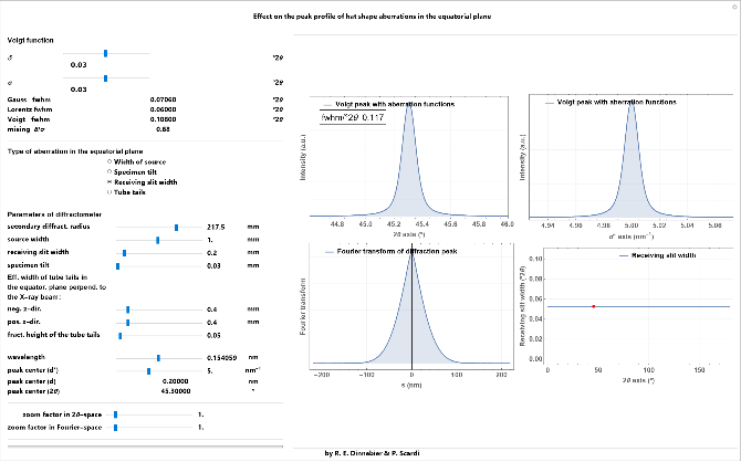
Effect on the peak profile of aberrations in the equatorial plane (hat shape function)
Effect on the peak profile of aberrations in the equatorial plane (hat shape function)
Convolution of the box function into a Voigt profile in real and Fourier space. Different kinds of aberrations in the equatorial plane of a diffractometer originating from receiving slit, size of the source, specimen tilt, and tube tails as a function of diffraction angle 2θ can be selected.
Code
Code
Interface (interactive version in the attached notebook)
Interface (interactive version in the attached notebook)
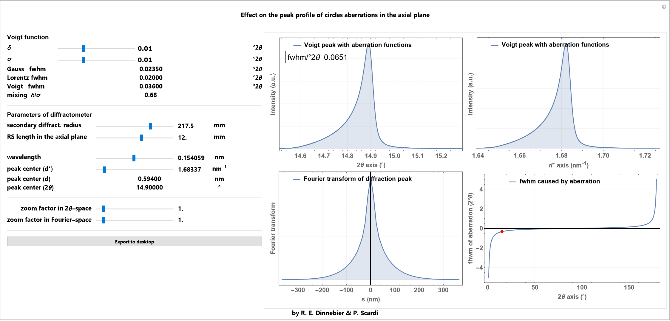
Effect on the peak profile of simple aberrations in the axial plane (circles function)
Effect on the peak profile of simple aberrations in the axial plane (circles function)
Convolution of the circles function into a Voigt profile in real and Fourier space. The aberration in the axial plane of a diffractometer originating from axial divergence caused by the length of a rectangular receiving slit as a function of diffraction angle 2θ can be selected.
Code
Code
Interface (interactive version in the attached notebook)
Interface (interactive version in the attached notebook)
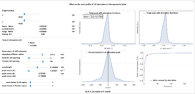
Effect on the peak profile of simple aberrations in the equatorial plane (1/X function)
Effect on the peak profile of simple aberrations in the equatorial plane (1/X function)
Convolution of the 1/x correction into a Voigt profile in real and Fourier space. The aberration due to equatorial divergence caused by either fixed or variable divergence slits as a function of diffraction angle 2θ can be selected.
Code
Code
Interface (interactive version in the attached notebook)
Interface (interactive version in the attached notebook)
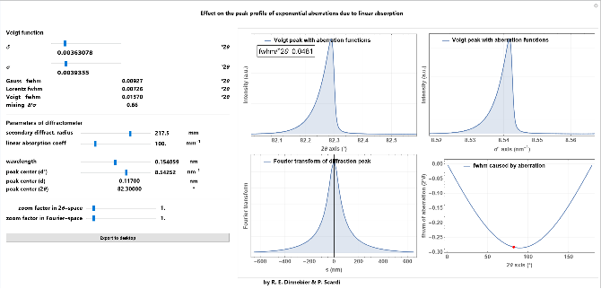
Effect on the peak profile of linear absorption (exponential function)
Effect on the peak profile of linear absorption (exponential function)
Convolution of the exponential correction function into a Voigt profile in real and Fourier space. The aberration due to the transparency effect caused by low linear absorption in flat plate samples holders with sample filled deep cavities is given as a function of diffraction angle 2θ.
Code
Code
Interface (interactive version in the attached notebook)
Interface (interactive version in the attached notebook)
In[]:=
Plot[{box[x,0.0,0.5]},{x,-0.5,0.5},PlotRangeFull,ExclusionsNone,GridLinesAutomatic,GridLinesStyleOpacity[.1],PlotStyle{Thick},FrameTrue,FrameLabel{"2θ (°)","normalized intensity","box (hat) function"},FrameTicks{{Automatic,None},{Automatic,Automatic}},LabelStyleDirective[Bold,16],FillingNone,PlotLegendsPlaced[LineLegend[{"fwhm = 0.5 °2θ"}],{0.45,Bottom}],TicksStyleDirective[Black,15],AxesStyleDirective[Black,Thick],ImageSize500]Plot[{halfbox[x,0.0,0.25]},{x,-0.5,0.5},PlotRangeFull,ExclusionsNone,GridLinesAutomatic,GridLinesStyleOpacity[.1],PlotStyle{Thick},FrameTrue,FrameLabel{"2θ (°)","normalized intensity","half box (hat) function"},FrameTicks{{Automatic,None},{Automatic,Automatic}},LabelStyleDirective[Bold,16],FillingNone,PlotLegendsPlaced[LineLegend[{"fwhm = 0.25 °2θ"}],{0.45,Bottom}],TicksStyleDirective[Black,15],AxesStyleDirective[Black,Thick],ImageSize500]Plot[{tubetail[x,0,0.3,-1,1.5,0.3]},{x,-2.5,2.5},PlotRangeFull,ExclusionsNone,GridLinesAutomatic,GridLinesStyleOpacity[.1],PlotStyle{Thick},FrameTrue,FrameLabel{"2θ (°)","normalized intensity","tube tail function"},FrameTicks{{Automatic,None},{Automatic,Automatic}},LabelStyleDirective[Bold,16],FillingNone,PlotLegendsPlaced[LineLegend[{"tubetails"}],{0.45,Bottom}],TicksStyleDirective[Black,15],AxesStyleDirective[Black,Thick],ImageSize500]Plot[{Re@ftbox[x,0.5],Im@ftbox[x,0.5]},{x,-100.,100.},PlotRangeFull,ExclusionsNone,GridLinesAutomatic,GridLinesStyleOpacity[.1],PlotStyle{Thick},FrameTrue,FrameLabel{"(2θ (°","Fourier transform","Fourier transform of box (hat) function"},FrameTicks{{Automatic,None},{Automatic,Automatic}},LabelStyleDirective[Bold,16],FillingNone,PlotLegendsPlaced[LineLegend[{"real part","imaginary part"}],{0.25,Top}],TicksStyleDirective[Black,15],AxesStyleDirective[Black,Thick],ImageSize500]Plot[{Re@fthalfbox[x,0.25],Im@fthalfbox[x,0.25]},{x,-100.,100.},PlotRangeFull,ExclusionsNone,GridLinesAutomatic,GridLinesStyleOpacity[.1],PlotStyle{Thick},FrameTrue,FrameLabel{"(2θ (°","Fourier transform","Fourier transform of half box (hat) function"},FrameTicks{{Automatic,None},{Automatic,Automatic}},LabelStyleDirective[Bold,16],FillingNone,PlotLegendsPlaced[LineLegend[{"real part","imaginary part"}],{0.25,Top}],TicksStyleDirective[Black,15],AxesStyleDirective[Black,Thick],ImageSize500]Plot[{ReceivingSlitWidth[x,0.1,217.5],SpecimenTilt[x,0.1,217.5]},{x,0.,180.},PlotRangeFull,GridLinesAutomatic,GridLinesStyleOpacity[.1],PlotStyle{Thick},FrameTrue,FrameLabel{"2θ (°)","fhwm of box function (°2θ)","aberrations in the equatorial plane"},FrameTicks{{Automatic,None},{Automatic,Automatic}},LabelStyleDirective[Bold,16],FillingNone,PlotLegendsPlaced[LineLegend[{"Size of source/ receiving slit width = 0.1 mm","speciment tilt = 0.1 mm"}],{0.45,Bottom}],TicksStyleDirective[Black,15],AxesStyleDirective[Black,Thick],ImageSize500]
-1
)
-1
)
-1
)
-1
)
The box function with a width of 0.5° 2θ on a 2θ scale and its real Fourier transform.
The half box function on a 2θ scale with a width of 0.25° 2θ and its complex Fourier transform.
Tube tail function as a combination of a box function and two (left, right) half box functions for the tails.
Aberrations in the equatorial plane of a diffractometer assuming a secondary radius of 217.5 mm, a slit width (either receiving slit or size of source) and a specimen tilt of 0.1 mm as a function of diffraction angle 2θ.
The circles function on a 2θ scale with three cut-off values of 2, 4, and 8° 2θ and the Fourier transform of the circles function with a cut-off value of 4° 2θ showing the real and the imaginary part.
Cut-off values (= curvature) of the circles function to describe asymmetry due to axial divergence as a function of scattering angle for a diffractometer with a secondary radius of 217.5 mm and different receiving slit lengths in mm.
The 1/x function on a 2θ scale with three cut-off values of 2, 4, and 8° 2θ and its Fourier transform with a cut-off value of 4° 2θ showing the real and the imaginary part.
Angular dependence of the 1/x correction function for modelling the peak asymmetry due to equatorial divergence caused by a fixed divergence slit of 0.5°, 1.0°, or 2.0° opening and a variable divergence slit with a constant illuminated sample length of 10 mm, 20mm, or 30 mm. The secondary diffractometer radius is set to of 217.5 mm.
The exponential function on a 2θ scale with three cut-off values of 2, 4, and 8° 2θ and its Fourier transform with a cut-off value of 4° 2θ showing the real and the imaginary part.