I’ve been given talks in the subject of Mathematical Games for awhile.
My next talk on Polygons and Polynomials will take place on Thursday, May 22nd at 11AM Chicago time.
My next talk on Polygons and Polynomials will take place on Thursday, May 22nd at 11AM Chicago time.
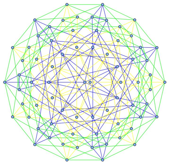
I use polygons all the time when I want something symmetrical. The latest example came from https://houseofgraphs.org/graphs/52273 and https://math.stackexchange.com/questions/5066009/classification-of-simple-finite-locally-c-7-graphs. How could we make that graph look good? But first, I found a nice embedding for a graph with local graph . I used polygons for initial symmetry, and then found polynomial roots to maximize the symmetry.
C
9
In[]:=
Graph[GraphData[{"NoncayleyTransitive",{28,13}}],VertexCoordinates->Join[Thread[{3,5,8,9,10,7,6,4,2}->(CirclePoints[9])],{1->{0,0}},Thread[{18,13,15,12,11,16,14,17,19}->Root[-1+3*#1+6*#1^2+#1^3&,2,0]CirclePoints[9]],Thread[{26,25,21,22,23,20,24,27,28}->Root[-1-6*#1-3*#1^2+#1^3&,2,0]CirclePoints[9]]]]
Out[]=
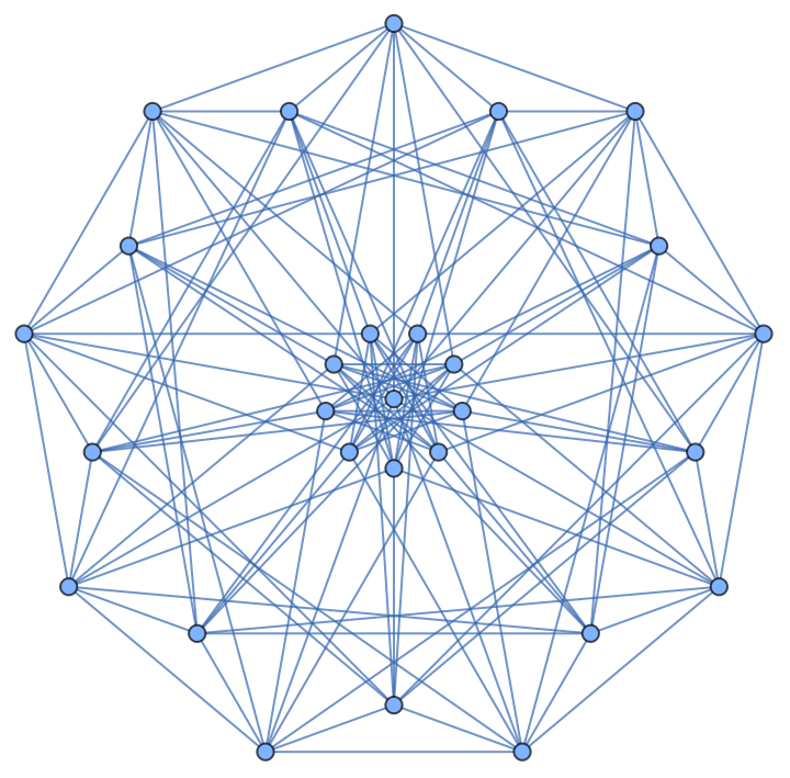
ee=;
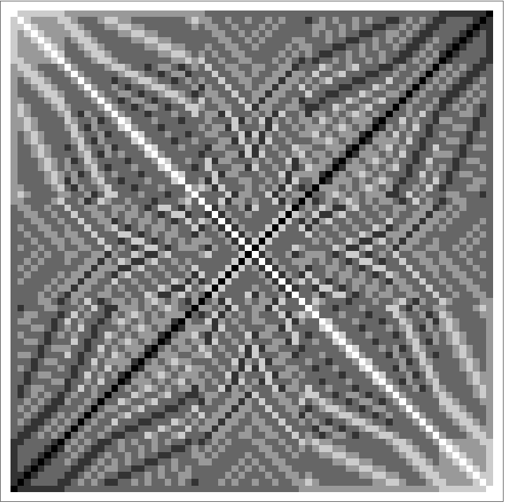
With this optimization, the graph distance matrix looks nice. The graph is locally
In[]:=
fmg=Graph[Range[72],UndirectedEdge@@@ee];gdm=GraphDistanceMatrix[fmg];ArrayPlot[gdm]
Out[]=
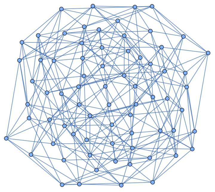
With just the edge list, the graph looks messy.
In[]:=
Graph[Range[36],UndirectedEdge@@@ee]
Out[]=
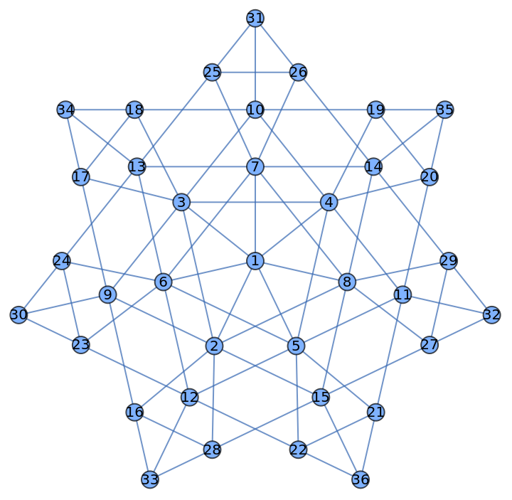
If we look at half of the graph, it has a nice structure that can be enhanced by polygons and polynomial roots. The other half of the graph looks identical. To see it, calculate 73-x for each vertex.
GraphRange[36],UndirectedEdge@@@Select[ee,Max[#]<=36&],VertexLabels->Placed[Automatic,Center],VertexSize->.3,VertexCoordinates->TakeThread->Flatten{{0,0}},CirclePoints[7],CirclePoints[7],CirclePoints[14],CirclePoints[7],1,36

Out[]=
With a bit of work, both halves of the graph can be put together.
In[]:=
Graph[Range[72],If[Max[List@@#]<=36,Style[#,Blue],If[Min[List@@#]>=37,Style[#,Yellow],Style[#,Green]]]&/@(UndirectedEdge@@@ee),VertexCoordinates->Join[{1->{0,0},72->{.2,0}},Thread[{6,68,4,70,2,65,7,67,5,69,3,71,8,66}->(1.35CirclePoints[14])],Thread[{9,58,14,60,12,62,10,64,15,59,13,61,11,63}->(2CirclePoints[14])],Thread[{24,23,51,52,20,19,55,56,16,28,46,44,26,25,49,50,22,21,53,54,18,17,57,45,27,29,47,48}->(2.47CirclePoints[28])],Thread[{30,37,35,39,33,41,31,43,36,38,34,40,32,42}->(3CirclePoints[14])]]]
Out[]=
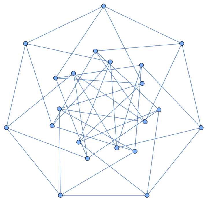
Another place I used polynomial roots and polygons is the braced heptagon:
In[]:=
GraphData[{"BracedHeptagon",{42,1}},"VertexCoordinates"]
Out[]=
,,,,,,0,,,,,,-,,,,,,,,,,,,,,,,,,,,,,,,,,,,,
1
2
1
2
This graph is so rigid that any two connected vertices can be completely ripped out and the graph will still be rigid. Oddly, I found this graph and got it into GraphData more than a decade before wondering if the graph might be rigid.
In[]:=
GraphData[{"BracedHeptagon",{42,1}}]
Out[]=
I also looked at polygons in origami. After making a new function for the Beloch Fold, I was amazed that the simple vertices of an equilateral triangle were enough for the construction of the nonagon.
If you’d like to see more, the talk on Polygons and Polynomials will take place on Thursday, May 22nd at 11AM Chicago time. Or just wait, I’ll be posting the full notebook here.
CITE THIS NOTEBOOK
CITE THIS NOTEBOOK
Polygons, polynomials and the Fricke-Macbeath graph
by Ed Pegg
Wolfram Community, STAFF PICKS, May 21, 2025
https://community.wolfram.com/groups/-/m/t/3465265
by Ed Pegg
Wolfram Community, STAFF PICKS, May 21, 2025
https://community.wolfram.com/groups/-/m/t/3465265