Abstract: The aim of this project was to develop the correspondence between statistical mechanics and multiway string substitution systems in the Wolfram Model. This was done by looking at various string rewrite rules and checking if they had any relation to statistical models, for example the Ising model. The change in the entropy of the system over iterations was checked and found that it does not always increase even in ‘closed’ systems. Different ways of defining configuration and phase space were also investigated, with a configuration space Lyapunov exponent found.
Introduction to statistical mechanics
Introduction to statistical mechanics
Statistical mechanics is usually studied in equilibrium where the passage of time is ignored,multiway graphs may allow for the study of dynamical/ non-equilibrium thermodynamic systems where each layer of updating events corresponding to a new moment in time, and by changing the rewrite rules and initial conditions of the multiway system many different systems can be simulated. The key example throughout this project was the 1D Ising model because of it’s simplicity and the fact that there is a known solution. The Ising Hamiltonian (Energy Function) is given by:where is the energy, is the coupling constant between spins (which are either 1 or -1), and is the magnetic field strength. The summation over means sum over all nearest neighbors applying periodic boundary conditions. Using the canonical ensemble one can find the probability of having a certain energy using:
H=-J-B
∑
<i,j>
s
i
s
j
∑
i
s
i
H
J
s
i
B
<i,j>
H
p(H)=exp(-βH)/Z,Z=exp(-βH(s))
∑
{s}
where β is the inverse temperature, and Z is the partition function which is found using the sum of the Boltzmann factors (exponentials) for every spin configuration. In 1D an exact solution for infinitely many spins is know and we aim to recreate it.
String substitutions and the Spin Flip Model
String substitutions and the Spin Flip Model
The easiest way to introduce string substitution systems is with an example. We start with the string “A” and apply the rule “A”→ “AB”, “B”->”BA”. The multiway graph for this is:
ResourceFunction["MultiwaySystem"][{"A""AB","B""BA"},"A",4,"EvolutionGraphFull",AspectRatio1/4]
Out[]=
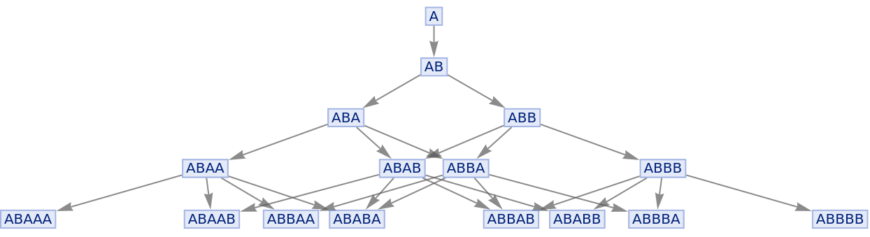
We see that the multiway system finds where it can apply any rule in the string and trees out every possible new string. At each layer of updating events we can take a horizontal slice to get a branchial graph that shows which strings came from the same common ancestor. We also define probability for a vertex on the branchial graph as the number of paths leading to it from the previous step, divided by the total number of paths from any vertex in the previous step to any vertex in the current step.
ResourceFunction["MultiwaySystem"][{"A""AB","B""BA"},"A",4,"BranchialGraph"]
Out[]=
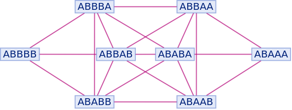
This rule was not chosen randomly and is what I call the ‘Spin Flip’ rule as for every letter in the string it produces the a new letter to the right which is the opposite. This was chosen for 3 reasons; if it is run forever it will produce strings of infinite length; the strings at each updating layer are the same length; and that it produces an opposite letter pair at every opportunity. This last reason is because in the 1D Ising model it is energetically favourable to produce these ‘domain walls’ and this rule causes them to proliferate.
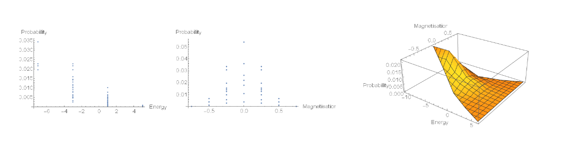
If this system is fun for several iterations we get a distribution of strings in the branchial graphs. We then find their energies by applying the Ising Hamiltonian to each one, find the magnetisation (average spin) and plot them against their probabilities. As expected we get an exponential distribution in energy with lower energy being more likely, we also get an approximate normal distribution for the magnetisation which is centred around zero. This is also predicted as the proliferation of these domain walls in the Ising model causes a zero magnetisation for temperatures >0. Although this system cannot be run easily for >10 iterations my prediction is that the magnetisation normal distribution will become narrower over iterations as the string’s approach infinite length. As a visual aid it may be helpful to plot these both together into a 3D plot as it shows the low energy, 0 magnetisation states are the most likely. The title plot is one of these 3D plots for a more complicated set of rules.
If this system is fun for several iterations we get a distribution of strings in the branchial graphs. We then find their energies by applying the Ising Hamiltonian to each one, find the magnetisation (average spin) and plot them against their probabilities. As expected we get an exponential distribution in energy with lower energy being more likely, we also get an approximate normal distribution for the magnetisation which is centred around zero. This is also predicted as the proliferation of these domain walls in the Ising model causes a zero magnetisation for temperatures >0. Although this system cannot be run easily for >10 iterations my prediction is that the magnetisation normal distribution will become narrower over iterations as the string’s approach infinite length. As a visual aid it may be helpful to plot these both together into a 3D plot as it shows the low energy, 0 magnetisation states are the most likely. The title plot is one of these 3D plots for a more complicated set of rules.
Out[]=
One problem is how to change the temperature or applied magnetic field of such a system, and one idea is to change the initial string in the system. If we repeat the procedure as above then an exponential can be fitted to the energy distribution giving us a β value, and a normal distribution can be fitted to the magnetisation with the mean giving the magnetisation of the whole system. We plot below to find some triangular distribution after 8 iterations.
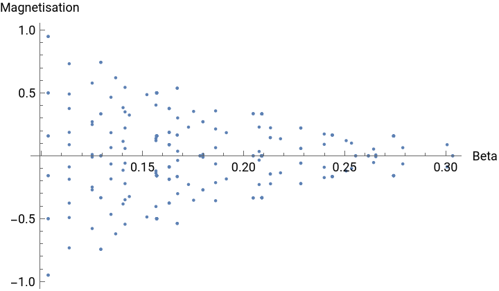
This seems promising as the lower the value of β the higher the magnetisation is, and as β increases the magnetisation comes closer to zero, with the hypothesis that after an infinite number of iterations the magnetization will be zero for all β > 0. This promise is quashed when we remember that β is inverse temperature and in fact the diagram show be flipped in the y axis for it to be correct. This does not destroy all hope for this model but does mean some better way of defining temperature must be found. One glaring problem with this way of defining temperature is that some initial strings will be contained within the multiway graph of another initial string and are not totally separate systems.
Rather than trying to explicitly define temperature for such string systems we could also just find the energies of the strings, their degeneracies (how many strings have the same energy), and plug the values into the formula for the partition function with β left as a variable. We then find the free energy density as -ln(Z)/βN, with N being the string length, and compare it to the known solution in zero field. Below shows the spin flip free energy at 2 and 8 iterations, and my prediction is that after infinite iterations they will exactly match. This can be done for other rules that do not have constant string length and they all seem to be converging as long as the rules create domain walls at every iteration.
Rather than trying to explicitly define temperature for such string systems we could also just find the energies of the strings, their degeneracies (how many strings have the same energy), and plug the values into the formula for the partition function with β left as a variable. We then find the free energy density as -ln(Z)/βN, with N being the string length, and compare it to the known solution in zero field. Below shows the spin flip free energy at 2 and 8 iterations, and my prediction is that after infinite iterations they will exactly match. This can be done for other rules that do not have constant string length and they all seem to be converging as long as the rules create domain walls at every iteration.
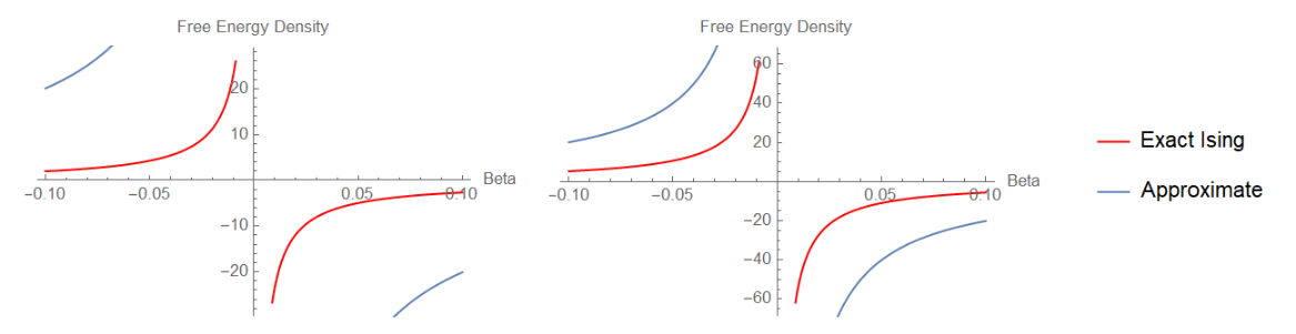
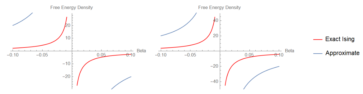
One could also do the same for rules that conserve string length such as the rule 30 cellular automaton, and below shows such a system at 2 and 4 iterations. This again seems to be converging and my reasoning for this is that the pseudo randomness of rule 30 effectively produces the many domain walls that are characteristic of the 1D ising model.
Entropy change
Entropy change
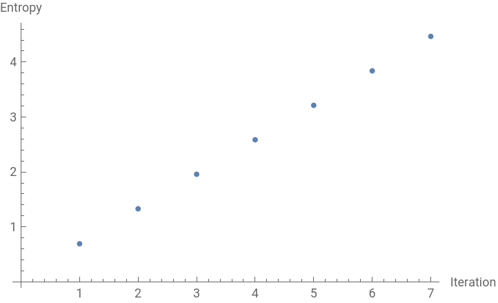
In statistical mechanics the entropy is given by ). By using the probabilities of the different nodes in the branchial graph we can calculate the entropy of each branchial graph and plot them over time to determine whether the system has a thermodynamic arrow of time. We find for the spin flip rule that entropy increases linearly over time with the rate of increase just less than the Shannon entropy, , with the increase being just less because although we are adding one bit of information at every iteration, not all states are equally likely, and some strings are never explored in this rule. This system exhibits a thermodynamic arrow of time as the entropy always increases.
S=-ln(
∑
i
p
i
p
i
ln2
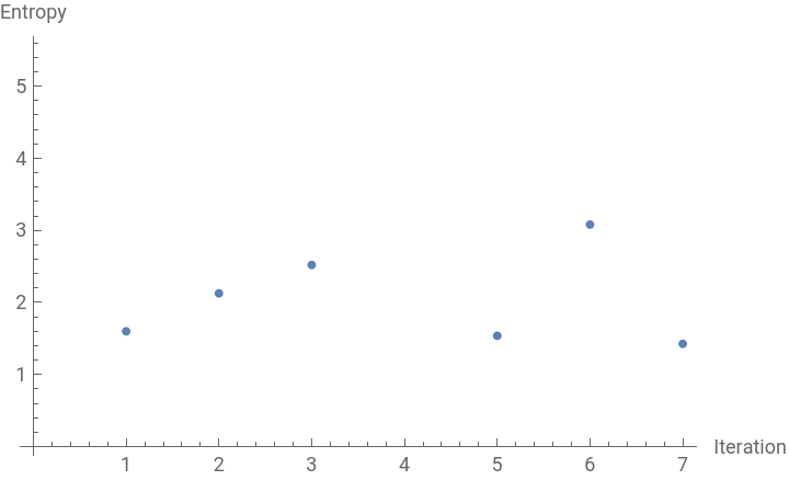
We may also want to consider the entropy increase for systems of fixed length such as multiway cellular automata, using rule 30 we find that entropy does not uniformly increase. This means we cannot treat all systems of constant length as being the same as closed systems in thermodynamics (i.e. having constant particle number) as in closed systems the entropy must always increase. The entropy change for a 5 bit string using rule 30 is shown below.
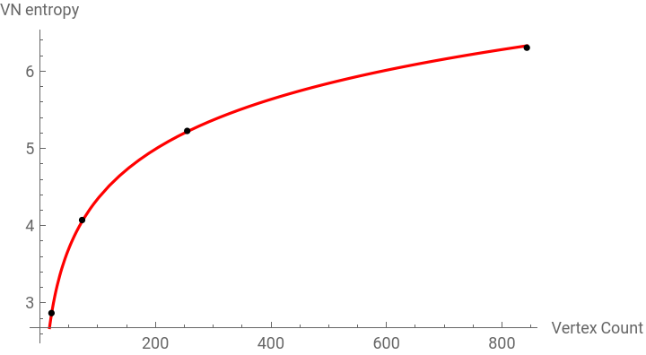
The statistical mechanical entropy has a quantum analogue, the Von Neumann entropy given by =Tr[ρlnρ] where ρ is the density matrices. This leads to the interpretation of the branchial graphs showing the time evolution of the density matrices. The time evolution is known to follow the Von Neumann equation which is the quantum analogue of the classical Liouville equation which governs how the phase space density of a collection of particles evolves over time. A multiway analogue of this could not be found and is left as an open question.One may also wonder how the entropy depends on the number of paths through the multiway graph, i.e. the number of vertices in each branchial graph. For a variety of different rules, even ones that do not produce strings of constant length at each iteration, we find that there is a logarithmic increase in entropy with the number of vertices. If this entropy represents the entanglement entropy of the nodes in the branchial graph then this may represent some form of area/volume law.
S
VN


Configuration Space and Lyapunov exponents
Configuration Space and Lyapunov exponents
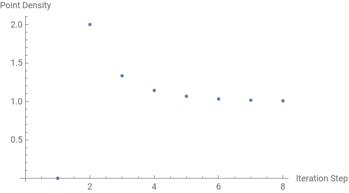
In ordinary classical mechanics the phase/ configuration space evolution of the system is of importance but it is not clear how to define one here. For a string of a given length N we have an N dimensional configuration space which cannot be easily visualised above N=3. We can ‘project’ this N dimensional space down to lower dimensions and one choice is where one dimension is the length of the string, and another is the binary to integer conversion. It may be of interest to look at the density of points in this configuration space over time (iteration step). This is shown below for the spin flip system which shows the density converging to one, i.e. every possible state in the configuration space of a string that length is eventually explored with equal likelihood.
2
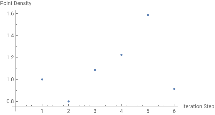
We can also do the same for cellular automaton multiway rules, and we show this for rule 30 below with a random 6 bit starting string and this system has a seemingly random density of points in the configuration space.
It is also interesting to see how such a configuration space evolves over time and we can do this for various rules. The animation below is for the spin flip rule but it is adapted so that it also flips the orientation of domain walls.
Future work
Future work
If this work was to be continued the key areas to focus on would be: How to define temperature and external field in such systems; how to create different statistical ensembles; proving the Von-Neumann/ Liouville equation in such systems; and finally relating the multiway graph to Euclidean path integrals in statistical physics.