In this project, I explore multi-way tag systems, an extension of the deterministic tag system model of computation invented by Emil Post. I implement algorithms to enumerate these systems and visualize their behavior, and I examine particular classes of these systems such as ones over singleton alphabets and ones which have only finitely many reachable states (from a given set of strings). Finally, I define two measures of the growth of multi-way tag systems, and implement methods to approximate or exactly compute these measures.
Introduction
Introduction
Tag Systems and Their Motivation
Tag Systems and Their Motivation
Tag systems are an extremely simple model of computation invented by Emil Post in the early twentieth century (Post, 1943). In trying to simplify the string-manipulation operations involved in the formal languages used to formalize mathematics, he came across a very simple construction. A tag machine transforms a string one operation at a time. At each step, a constant number (called the deletion number) of symbols are removed from the beginning of the string, and depending on the first of those symbols something is appended to the end of the string.
Post tried for months to understand the behavior of just one of these systems: cut off three symbols from the start, then add ‘00’ to the end if the first symbol (before being cut off) was a 0 or ‘1101’ if the first symbol was a 1. To this day, it is not known whether there are strings which grow forever . These apparently simple systems proved to have surprisingly complex behavior. In fact, they were later even shown to be Turing-complete (Cocke & Minsky, 1964).
Multi-Way Tag Systems
Multi-Way Tag Systems
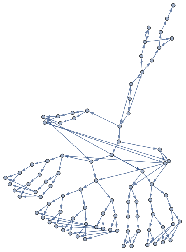
One extension to tag systems is to allow the production rules mapping symbols to appended strings to be non-deterministic. For example, what if strings starting with 0 could become ‘1011’ as well as Post’s original ‘1101’? One way to visualize this is to draw a multiway graph where each vertex represents a string and edges represent the system’s transformation of one string into another. For example, we can graph how the above extension to Post’s original tag system can evolve within ten steps from the string ‘100’.
Hovering over the vertices will show the strings to which they correspond.
In[]:=
stateGraphPlot[{v->3,0->{0,0},1->{1,1,0,1},1->{1,0,1,1}},{{1,0,0}},10,GraphLayout->{"RadialEmbedding","RootVertex"->{1,0,0}}]
Out[]=
Wolfram Language Implementation
Wolfram Language Implementation
I’ll write system specifications as lists of rules in the following form, with one rule mapping to the deletion number, and the rest mapping symbols to strings.
v
postSystem = {v -> 3, 0 -> {0, 0}, 1 -> {1, 1, 0, 1}};multiPostSystem = postSystem ~Join~ {1 -> {1, 1, 1, 0}, 1 -> {0, 1, 1, 1}, 1 -> {1, 0, 1, 1}};rabbitSystem = {v -> 1, 0 -> {0}, 0 -> {1, 0}, 1 -> {}};
Then, I’ll implement evolution of multi-way tag systems by transforming system specifications to replacement rules.
In[]:=
systemToReplacementRules[system:{v -> v_Integer, productionSpec___}] := {productionSpec} /. HoldPattern[head_ -> tail_List] :> Flatten[{head, ConstantArray[_, v - 1], w___}] :> Join[{w}, tail]evolveSystem[system_List] := evolveSystem[system, #]&evolveSystem[system_List,state_List] := Flatten[ReplaceList[systemToReplacementRules[system]] /@ state, 1]
Now we can plot a graph of how these systems evolve:
In[]:=
stateGraph[system_List, init_List, maxIters_:Infinity] := ResourceFunction["FixedPointGraph"][ReplaceList[systemToReplacementRules[system]], init, maxIters]stateGraphPlot[system_List, init_List, maxIters_:Infinity, opts:OptionsPattern[]] := GraphPlot[ stateGraph[system, init, maxIters], VertexLabels -> v_ :> Placed[StringJoin @@ ToString /@ v, Tooltip], opts]stateGraphPlot3D[system_List, init_List, maxIters_:Infinity, opts:OptionsPattern[]] := GraphPlot3D[ stateGraph[system, init, maxIters], VertexLabels -> v_ :> Placed[StringJoin @@ ToString /@ v, Tooltip], opts]
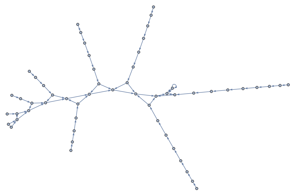
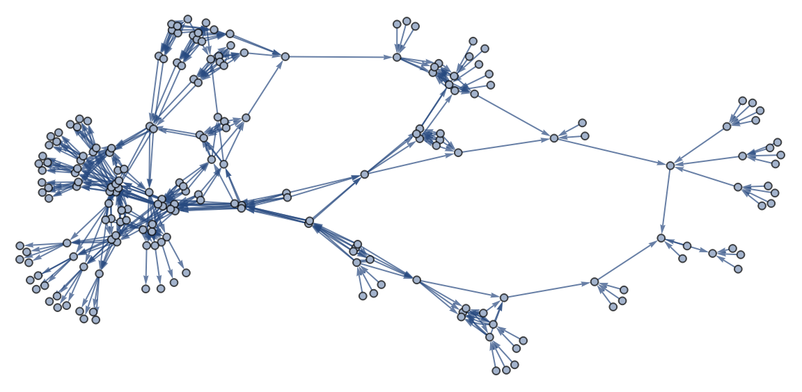
For example, here are graphs of two different multi-way tag systems. On the left is a system I call the “rabbit system” for reasons we’ll see later, and on the right is a multi-way extension of Post’s original system.
In[]:=
Row[{stateGraphPlot[rabbitSystem,Flatten[Permutations[Prepend[ConstantArray[1,#],0]]&/@Range[9],1],3,ImageSize->Large],stateGraphPlot[multiPostSystem,Flatten[Tuples[{0,1},#]&/@Range[3,6],1],3,ImageSize->Large]}]
Out[]=
The Landscape
The Landscape
Enumeration of Tag Systems
Enumeration of Tag Systems
To get an idea of how these systems behave, I’ve implemented a function that lists every possible tag system with a certain deletion number, alphabet, rule count, and maximum append length.
In[]:=
enumerateSystems[del_Integer, abc_List, rules_Integer, suf_Integer] := Module[{ruleLhsLists, ruleRhsLists, productionSpecs}, ruleLhsLists = Flatten @* MapIndexed[ConstantArray[abc[[#2]], #1]&] /@ IntegerPartitions[rules, {Length[abc]}]; ruleRhsLists = Tuples[Flatten[Tuples[abc, #]& /@ Range[0, suf], 1], rules]; productionSpecs = Flatten[Table[Thread[lhsList -> rhsList], {lhsList, ruleLhsLists}, {rhsList, ruleRhsLists}], 1]; DeleteDuplicates[Prepend[v -> del] @* Sort /@ productionSpecs]]
For example, we can count the number of binary tag systems “at least as simple” as Post’s original tag system by looking at all the binary tag systems with only two rules and adding at most four symbols to the end in each rule.
In[]:=
enumerateSystems[2,{0,1},2,4]//Length
Out[]=
961
Let’s take a look at some of the simplest tag systems, with only one symbol.
Singleton Alphabets and Linear Diophantine Equations
Singleton Alphabets and Linear Diophantine Equations
If there’s only a single symbol in the alphabet, then words are completely determined by their length. In this case, tag operations simply change the length of the word by adding an integer value. For example, the tag system defined by can either subtract one or add two at each iteration. This gives us that the language of strings generated by the system from the initial string is , where satisfies the Diophantine equation with . In general, any tag system with only one symbol in its alphabet can be rewritten as a linear Diophantine equation (in one variable, for deterministic tag systems).
v3,000,000000
s
a
n
a
n
xs-p+3q
p,q≥0
Here are state graphs for ten of the simplest tag systems over the alphabet , with edges labeled and colored according to how they affect the length of the string.
{0}
In[]:=
Row[stateGraphPlot[#,{{0,0}},4,GraphLayout->"LayeredEmbedding",EdgeLabels->{x_y_:>NumberForm[Length[y]-Length[x],NumberSigns->{"-","+"}]},EdgeStyle->{x_y_:>Hue[0.3*(Length[x]-Length[y])]},ImageSize->Small]&/@enumerateSystems[2,{0},2,4],Spacer[30]]
Larger Alphabets
Larger Alphabets
Systems over larger alphabets exhibit much more complex behavior. We’ll start by enumerating the smallest class of systems with a binary alphabet and one non-deterministic rule.
A lot of these tag systems are uninteresting in the sense that they either always grow strings or always shrink strings. Let’s look at systems with some rules that shrink and some that grow. This greatly reduces the number of systems, to just 708.
Press the “Show Animation Controls” button next to the sliders to enter in a number exactly.
Growth of Multi-Way Tag Systems
Growth of Multi-Way Tag Systems
Examining Growth
Examining Growth
Now, within this big space of 1800 tag systems, we want to find systems with interesting behavior. One thing that might be interesting is to measure how fast the number of unique strings grows.
We can start by plotting how the number of unique strings produced by the system grows as we continue applying the production rules. It’s very common for these systems to grow exponentially, so I’ve used a logarithmic scale.
As we can see, there are a lot of roughly exponential systems (linear, on the log plot) and finite systems which only ever reach a finite set of strings (horizontal lines, on the plot). What’s most interesting, though, are the ones in between the two extremes. I’ll now randomly select and examine some systems which appear to grow subexponentially on the above plot.
The Twin Horn System
The Twin Horn System
One of the systems I found this way is defined as
Click and drag to rotate the graph.
Examining the vertices in each horn (pause now to check the tooltips for each vertex above to find the pattern yourself, if you want) reveals that each one corresponds to the parity of the position of the first ‘1’ in the string.
Anyway, let’s plot the growth of the system as a function of time, but this time on a linear scale.
And fitting a line too it, we find that on average about two new strings are reached with each iteration.
Exponential Growth
Exponential Growth
I also looked at some of the fastest-growing dynamic systems. In particular, the system defined by
Again graphing the growth in each iteration, we can pretty clearly see an exponential trend.
So it appears that this system has a state growth rate of about 1.22, at least around fifty iterations.
Path Growth Rate and Natural Selection
Path Growth Rate and Natural Selection
The trivial implementation of this is extremely similar to the implementation of state growth rate, but without the deletion of duplicate strings at each iteration.
And we can use this to estimate the path growth rate of our simple fast-growing system to be about 1.52, at least after thirty iterations. Unfortunately, because the number of strings grows exponentially it becomes exponentially more resource-intensive to compute the path growth rate this way. Thankfully, there is a linear time algorithm that can accurately estimate it.
The key insight that leads to this algorithm is that this process is in a sense similar to natural selection. We start out with an initial population of strings which then reproduces via the tag operations to create new strings. Since we’re taking the limit as the number iterations goes to infinity, we ultimately care only about the “species” of strings which can reproduce at the greatest rate. In the full fidelity estimation, there is no “competition” among strings — they all live forever, taking up compute resources in each iteration. Instead, we can limit the number of strings in each iteration by taking a random sample from the offspring of the last iteration. Notably, this (usually) does not change the result, because the strings which reproduce fastest are more likely to be included in the sample and will therefore usually outcompete other “species” of strings.
I’ll now verify that this works by running 100 trials of 1000 iterations each with a max population size of 50, and plotting a histogram of the resulting computed growth rates.
Graph Eigenvalues and Rabbits
Graph Eigenvalues and Rabbits
It is also possible to compute the path growth rate efficiently and exactly for multi-way tag systems that are “finite” in the sense that only a finite number of states are reachable from their initial state.
For example, consider the following tag system, which I call the “rabbit system:”
Beginning with the initial string ‘0’, the state graph contains just two elements, ‘0’ and ‘10’:
Wait, isn’t that the golden ratio? What’s going on here? Let’s list out the number of paths in each iteration.
It’s also possible to compute the path growth rate similarly to how one can analyze the long-term behavior of a discrete-time Markov chain. As in a Markov process, the long-term behavior is dominated by the effects of the principal eigenvalue of the adjacency matrix (analogous to the transition matrix for a Markov chain). Specifically, I conjecture that the path growth rate is the value of the largest eigenvalue corresponding to an eigenvector not orthogonal to the initial path count vector. For example, the rabbit system has path growth rate equal to
Which is exactly the golden ratio.
Conclusions
Conclusions
In this essay, I have implemented an algorithm to enumerate all possible multi-way tag systems. I’ve also begun to explore this expansive space, examining in detail a few systems and classes of systems. Systems over alphabets with only one symbol can be reduced to linear Diophantine equations. For systems of more than one variable, I’ve defined two notions of growth rate, the state growth rate and path growth rate, and used these to find and examine some interesting examples of multi-way tag systems.
Future Directions
Future Directions
I conjecture that multi-way tag systems are equivalent in power to non-deterministic Turing machines in the sense that any non-deterministic Turing machine can be efficiently simulated by some multi-way tag system. Unfortunately, constructing such a tag system is very difficult because one Turing machine operation will consist of many tag operations, so any combination of non-determinism in those many tag operations must result in a valid Turing machine operation.
It would also be interesting to more formally define the state and path growth rates, and examine whether there are more efficient methods to compute them for tag systems with infinite state graphs.
Appendix: Complexity of 1-Tag Systems
Appendix: Complexity of 1-Tag Systems
It can be useful to think of tag systems not as a model of computation but rather as a class of very simple formal grammars, as Post originally did (Post, 1943). This allows us to examine the behavior of tag systems using the tools of formal languages. One thing we can do is classify the complexity of tag systems based on their position in the Chomsky hierarchy of languages.
One conjecture I had was that 1-tag systems, which delete only one symbol at a time, would contained within the class of context-free languages. This is in contrast to tag systems which delete two or more symbols, which are in the much more complex class of recursively enumerable languages by virtue of their Turing-completeness. However, this conjecture proved to be false.
As a counterexample, let’s look at the 1-tag system defined by the following rules:
That is, the first symbol of the string is doubled and moved to the end of the string, unless it’s a b in which case it’s simply moved to the end without being doubled.
Starting with the string ‘ab’, let’s look at how the system evolves:
Starting with the string ‘ab’, let’s look at how the system evolves:
References
References
◼
Bar-Hillel, Y., Perles, M., and Shamir, E. (1961). On formal properties of simple phrase structure grammars. Zeitschrift für Phonetik, Sprachwissenschaft und Kommunikationsforschung, 14:143–172. Reprinted in Bar-Hillel, Y. (1964). Language and Information: Selected Essays on their Theory and Application, Addison-Wesley 1964, 116–150.
◼
Cocke, J., & Minsky, M. (1964). Universality of tag systems with P = 2. Journal of the ACM, 11(1), 15–20. https://doi.org/10.1145/321203.321206
◼
Post, E. L. (1943). Formal Reductions of the General Combinatorial Decision Problem. American Journal of Mathematics, 65(2), 197–215. https://doi.org/10.2307/2371809
◼
Wikipedia contributors. (2024, July 9). Fibonacci sequence. In Wikipedia, The Free Encyclopedia. Retrieved 16:12, July 11, 2024, from https://en.wikipedia.org/w/index.php?title=Fibonacci_sequence&oldid=1233560077
Acknowledgements
Acknowledgements
CITE THIS NOTEBOOK
CITE THIS NOTEBOOK
Growth and evolution of multi-way tag systems
by Max Niederman
Wolfram Community, STAFF PICKS, July 12, 2024
https://community.wolfram.com/groups/-/m/t/3216229
by Max Niederman
Wolfram Community, STAFF PICKS, July 12, 2024
https://community.wolfram.com/groups/-/m/t/3216229