This contribution is the second one in the author’s series focusing on reproducibility of milestone results in mathematical chemistry with the help of Wolfram Language. The first contribution was a recent example published by the author about partial ordering of boiling points of alkanes, whereas in this case the focus will be on Chapter 13 “Graphical Bioinformatics” from the book “Solved and Unsolved Problems of Structural Chemistry” by Milan Randić, Marjana Novič and Dejan Plavšić, CRC Press (2016). A basic graphical method will be presented for visualizing and comparing DNA sequences belonging to different animal species [1, 2]. The final step will be the derivation of the phylogenetic tree from invariants of the input DNA sequences without resorting to their reciprocal alignment, which is the standard base method for comparing sequences, nowadays. The field of graphical bioinformatics is quite novel and comprises a variety of creative methods [3]. Among these, the Chaos Game Representation stands out historically as the most prominent in scientific literature, as shown in this recent review [4]. However, the procedure shown here based on dual maps with Four-Color coding can be followed very easily also by first-year undergraduates and non-experts in bioinformatics, since it only requires basic linear algebra notions, such as matrices and eigenvalues. It can even be introduced with some simplifications about eigenvalue concept to K-12 students. While the method is very simple in its foundations, the computational implementation requires a careful mastery of computational geometry functions provided by the Wolfram Language (2D meshes, graphs and Euclidean distance matrices), especially as far as mesh adjacencies are considered in particular situations. Nonethless, the overall procedure can be very useful to grasp the machinery behind the construction of phylogenetic trees from sequence datasets.
Method Outline
Method Outline
The basic idea behind the Four-Color map representation of DNA by Milan Randić and co-authors is to transform a 1D object (i.e. the DNA letter sequence with A, C, T and G bases) into a 2D object or template with square tessellations where each DNA base is placed with a predefined color. Other templates are also possible with triangular or hexagonal tilings [2]. This procedure allows for minimization of local variations in the DNA sequences when they are compared, so that all global changes are retained. For simplicity, the square tessellation in 2D will be chosen as reference mapping scheme in this post. After setting the DNA sequence in a spiral shape, one obtains a 2D array of square cells labelled according the four DNA bases, represented by letters A, C, T and G, which can be conversely identified with four colors. By merging adjacent cells sharing the same label or color into a single super-cell, one obtains a simpler 2D map where macro-regions having the same nucleotide base can be identified with the same color. This step lowers the dimensionality of the matrix problem, since the number of cells is of course reduced after the merging process. Then, dual graphs can be constructed by replacing the centroid of each super-cell with a vertex embedded in the 2D (x,y) coordinate framework and connecting vertices of adjacent super-cells. The last step is the numerical characterization of the obtained dual graphs, which makes graphical bioinformatics a truly quantitative approach. Since dual graphs, in contrast to ordinary graphs, are embedded in 2D the (x, y) plane where all vertices have fixed positions and edges have fixed lengths, one can resort to the eigenvalue computation of the squared Euclidean distance matrix built on the graph vertices. This is a very intriguing aspect of the proposed method, since these mathematical data structures always have four nonzero eigenvalues (one positive and three negative) independently from the matrix size. This actually allows for the comparison of sequences of different lengths and therefore the construction of the phylogenetic tree for different species.
Setting the DNA sequence in a square spiral pattern
Setting the DNA sequence in a square spiral pattern
The starting point of the procedure is to obtain the DNA sequences for a given set of species. As a general example to be checked against the reference literature (Fig. 13.3 in [1] and 1 in [2]) , the DNA sequence of the first exon of β-globin gene of Cattle (Bos taurus) will be chosen.
In[]:=
(*Cattle(Bostaurus)firstexonofβ-globingene*)CattleDNAMR="ATGCTGACTGCTGAGGAGAAGGCTGCCGTCACCGCCTTTTGGGGCAAGGTGAAAGTGGATGAAGTTGGTGGTGAGGCCCTGGGCAG";Characters[CattleDNAMR]//Length
Out[]=
86
In order to draw the square spiral pattern the code from George Beck’s contributed SquareSpiralPoints function in the Wolfram Function Repository can be used, which is reported here for commodity
In[]:=
SquareSpiralPoints[n_]:=AnglePath[Join@@(Prepend[#1,90]&)/@Table[0*Range[k/2],{k,0,n-1}]*Degree]
In[]:=
spiral=SquareSpiralPoints[18]
Out[]=
{{0,0},{0,1},{-1,1},{-1,0},{-1,-1},{0,-1},{1,-1},{1,0},{1,1},{1,2},{0,2},{-1,2},{-2,2},{-2,1},{-2,0},{-2,-1},{-2,-2},{-1,-2},{0,-2},{1,-2},{2,-2},{2,-1},{2,0},{2,1},{2,2},{2,3},{1,3},{0,3},{-1,3},{-2,3},{-3,3},{-3,2},{-3,1},{-3,0},{-3,-1},{-3,-2},{-3,-3},{-2,-3},{-1,-3},{0,-3},{1,-3},{2,-3},{3,-3},{3,-2},{3,-1},{3,0},{3,1},{3,2},{3,3},{3,4},{2,4},{1,4},{0,4},{-1,4},{-2,4},{-3,4},{-4,4},{-4,3},{-4,2},{-4,1},{-4,0},{-4,-1},{-4,-2},{-4,-3},{-4,-4},{-3,-4},{-2,-4},{-1,-4},{0,-4},{1,-4},{2,-4},{3,-4},{4,-4},{4,-3},{4,-2},{4,-1},{4,0},{4,1},{4,2},{4,3},{4,4},{4,5},{3,5},{2,5},{1,5},{0,5},{-1,5},{-2,5},{-3,5},{-4,5},{-5,5}}
In[]:=
Length[spiral]
Out[]=
91
For reproducing exactly the orientation of the example picture reported in Fig. 13.3 of Ref.[1] or equivalently Fig.1 in Ref.[2], the spiral needs to be rotated and mirrored, besides being shortened by 5 points to match exactly the DNA sequence length as follows
rot=RotationTransform[Pi/2];mirror=ReflectionTransform[{0,-1}];p1=ListPlotmirror[rot[{Drop[spiral,-5]}]],
Out[]=
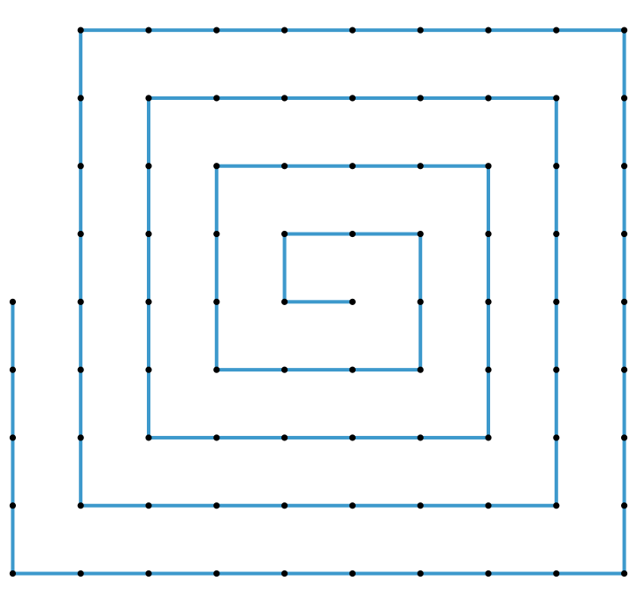
Next the obtained spiral points need to be sorted out and each point position within the spiral is mapped on a square-like 2D mesh array (e.g. in this case the first point in the spiral origin will be found at position 42 in the array). This step is crucial for assigning correctly all spiral points (hence letters) to the 2D matrix.
In[]:=
sortedspiral=Sort[Sort[Flatten[mirror[rot[{Drop[spiral,-5]}]],1],(#1[[1]]>#2[[1]])&],(#1[[2]]>#2[[2]])&];
In[]:=
positionsspiral=Flatten[Table[Position[Flatten[mirror[rot[{Drop[spiral,-5]}]],1],sortedspiral[[i]]],{i,1,Length[sortedspiral]}],2];
Check example: first point in spiral origin is found at position 42
In[]:=
positionsspiral[[42]]
Out[]=
1
In[]:=
spiralidx=Map[{#}&,positionsspiral];
In[]:=
lettseq=StringPartition[StringTake[CattleDNAMR,Length[Characters[CattleDNAMR]]],1];
DNA sequence with re-ordered spiral coordinates
In[]:=
spiralidxDNA=Extract[lettseq,spiralidx]
Out[]=
{G,G,A,T,G,A,A,G,T,T,A,C,C,G,C,C,T,T,G,C,G,A,G,G,A,T,G,A,T,T,G,C,T,G,T,G,G,A,G,C,T,A,G,A,T,T,A,A,C,G,T,C,A,A,G,G,C,G,C,G,T,C,G,G,G,G,G,T,G,G,A,A,C,G,G,T,G,G,T,C,C,C,G,G,A,G}
Construction of the mesh region
Construction of the mesh region
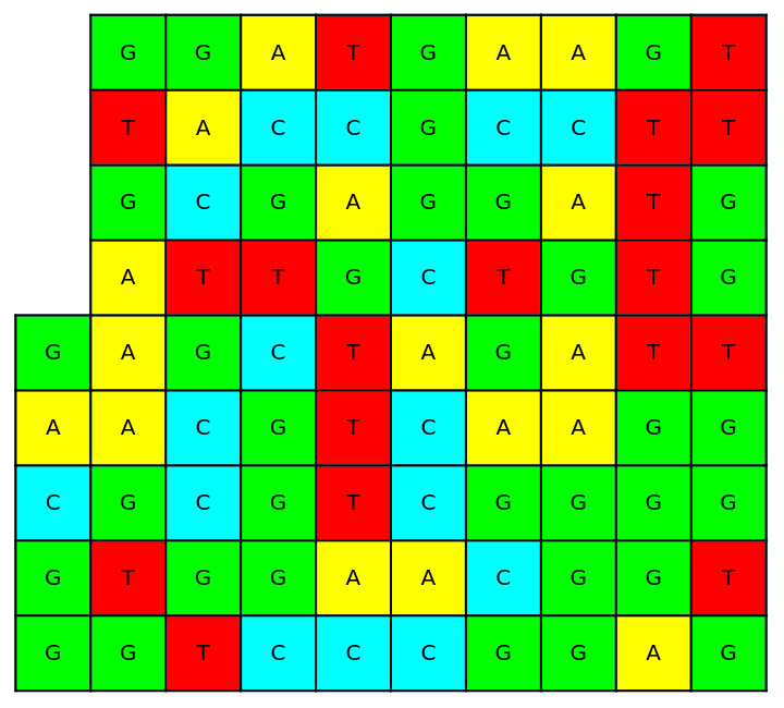
The following code allows to build a 2D mesh region to match the spiral orientation with all DNA sequence letters placed correctly to match the example reported in literature for Cattle [1, 2].
(*mesharraywith86elementstomatchthechosenDNAsequence*)arr86=Flatten[{Table[Flatten[{ConstantArray[0,{1}],ConstantArray[1,{9}]}],{4}],ConstantArray[1,{5,10}]},1];reg86=ArrayMesh[arr86];reg86spiral=ArrayMesh[arr86,MeshCellLabel->Table[MeshCells[reg86,2][[i]]->spiralidxDNA[[i]],{i,1,Length[Characters[CattleDNAMR]]}]];reg86spiralcolor=ArrayMesharr86,
Out[]=
Exercises
Exercises
The reader can try to adapt the above code lines to build and visualize the 2D mesh array for other species with different sequence lengths, such as Human (Homo sapiens) or Gorilla (Gorilla gorilla) with 92 and 93 characters, respectively. Just pay attention that one and two points must be added at the left-top corner of the spiral, respectively.
The reader is invited to build 2D arrays mapped onto triangular and hexagonal spirals, as reported in the cited paper [2].
Merging of adjacent mesh cells with same nucleotide label and visualization of the new mesh region
Merging of adjacent mesh cells with same nucleotide label and visualization of the new mesh region
From here on a lengthy procedure will be outlined to merge adjacent mesh cells in the obtained 4-color region having the same label (color).
First one needs the list of adjacent cells with same label for each considered cell in the mesh region.
First one needs the list of adjacent cells with same label for each considered cell in the mesh region.
jcells=Table[{(*indexofselected2Dcell*)midx=MeshCellIndex[reg86spiralcolor,MeshCells[reg86spiralcolor,2][[idx]]];(*correspondinglabeli.e.DNAbase*)mlab=AnnotationValue[{reg86spiralcolor,MeshCells[reg86spiralcolor,2][[idx]]},MeshCellLabel];(*adjacentcellsofselected2Dcell*)amc=AdjacentMeshCells[reg86spiralcolor,MeshCells[reg86spiralcolor,2][[idx]],2];(*findindicesofadjacentcellssharingsamelabel*)macpos=Position[StringMatchQ[AnnotationValue[{reg86spiralcolor,amc[[;;]]},MeshCellLabel],ToString[mlab]],True];(*listofcellstobejoinedintoaunifiedcellwithsamelabel*)exc=Extract[amc,macpos];Join[midx,exc]},{idx,1,Length[Characters[CattleDNAMR]],1}];
The duplicate sublists with indexes in swapped order need to be deleted as follows
In[]:=
(*deleteduplicatesadjacentcellsinswappedorder*)jcellssingle=DeleteDuplicates[Flatten[jcells,1],#1Reverse[#2]&];
Since there are still sublists with repeated cell indexes one can resort to graph theory to simplify repetitions by using SimpleGraph function, which deletes repeated edges (i.e. cell adjacencies)
In[]:=
ajc=jcellssingle[[;;,All,2]];g=Graph[Flatten[Table[Map[UndirectedEdge[First[ajc[[i]]],#]&,ajc[[i]]],{i,1,Length[ajc]}]]];gs=SimpleGraph[g];
Finally, the following lines allow to obtain the list of adjacent mesh cells sharing the same label, to be merged together into super-cells
In[]:=
conncells=ConnectedGraphComponents[gs];dataconncells=Table[VertexList[conncells[[i]]],{i,1,Length[conncells]}]
Out[]=
{{64,63,74,65,84,75,55,66,83,56},{26,17,35,18,45,9,46},{70,60,69,50},{48,38,47,28},{14,23,5,24},{82,81,80},{53,54,44},{51,41,61},{77,67,78},{16,15},{6,7},{29,30},{12,13},{36,27},{52,62},{71,72},{2,1},{59,49},{4},{85},{40},{31},{58},{10},{25},{3},{32},{37},{11},{57},{33},{8},{43},{86},{20},{19},{22},{21},{68},{34},{39},{73},{42},{76},{79}}
The new mesh region with merged cells can be constructed as a collection of different BoundaryMeshRegions where labels, colors and super-cell indexes have been newly defined and computed besides the centroids of each super-cell, which will be very useful in the final section. Let’s stress that the problem dimension now has reduced from 86 elements to 44 after merging of the same-color adjacent cells.
In[]:=
mlabsmerg=Table[First@Map[AnnotationValue[{reg86spiralcolor,MeshCells[reg86spiralcolor,#]},MeshCellLabel]&,Map[{2,#}&,dataconncells[[i]]]],{i,1,Length[dataconncells]}];mcolors=ReplaceAll[mlabsmerg,{"A"->Yellow,"C"->Cyan,"G"->Green,"T"->Red}];finmesh=Table[BoundaryMeshRegion[RegionUnion[MeshPrimitives[reg86spiralcolor,MeshCells[reg86spiralcolor,Map[{2,#}&,dataconncells[[i]]]]]],MeshCellStyle{{2}mcolors[[i]]}],{i,1,Length[dataconncells]}];meshcentr=RegionCentroid/@finmesh;im=Show[{finmesh,Graphics[Table[Text[i,meshcentr[[i]]],{i,1,Length[meshcentr]}]]}]
Graph construction of DNA dual maps
Graph construction of DNA dual maps
Now one needs to find the indexes of adjacent cells for each super-cells in order to build the final dual graph, of course again by avoiding mirror duplicates. In this case one can looks for any intersection of the boundary of each BoundaryMeshRegion with the surrounding ones.
Each vertex can be associated with the corresponding super-cell centroid and the undirected graph of cell adjacencies can be easily built and visualized as the so called dual map graph with its vertices and the corresponding nucleotide labels centered on the centroids
Eigenvalues of Euclidean Distance Matrices of dual graphs
Eigenvalues of Euclidean Distance Matrices of dual graphs
The numerical characterization of the above obtained dual graph can be accomplished by feeding the function DistanceMatrix with the super-cell centroid coordinates and the relevant option for squared Euclidean distance function.
As clearly pointed out in [1, 2] and references therein, such matrices show very interesting properties as far as diagonalization is concerned. Actually, one can see that only four nonzero eigenvalues are always obtained in the 2D case, regardless of matrix dimension. This is a special case of a more general property of Euclidean Distance Matrices (EDMs), when their individual matrix elements are raised to higher powers. When elements of an Euclidean distance matrix are raised to the second, third, fourth and fifth powers and so on, the number of non-zero eigenvalues of such matrices are 4, 9, 16, 25 and so on, correspondingly. Additionally, when Euclidean matrices in higher dimensions are considered (i.e. 3D, 4D, 5D), for the case of the squared matrix elements one obtains five, six and seven non-zero eigenvalues, respectively. Among these, one eigenvalue is always positive while the remaining ones are all negative.
Exercise
Exercise
The reader can check the above summarized linear algebra facts by constructing dual graphs for DNA sequences of different lengths, with EDMs elevated to square or higher powers, by using the DNA sequences reported in the cited literature [1, 2].
Construction of the phylogenetic tree from eigenvalues of dual maps
Construction of the phylogenetic tree from eigenvalues of dual maps
In the following, the reader can find the complete dataset of the eigenvalues of the dual maps for all the species considered in [1, 2] obtained by following the procedure above applied to DNA sequences of different animals. All the four-eigenvalue sets will be used for the construction of the phylogenetic tree of similarities among species, based on the option NormalizedSquaredEuclideanDistance used within Dendrogram or ClusteringTree
Incidentally, the author would like to point out that this tree is different from the (unreported) outcoming tree obtained from the four-eigenvalue dataset reported for the nine animal species in Refs. [1, 2]. In such case, the original dual graphs reported in literature slightly differ in the position of one or two vertices, which could be related to numerical issue with centroid computation method, which is however undocumented alongside the programming language.
In the present case, the reported computational procedure is totally reproducible and actually stems from exactly the same four-color 2D patterns as those reported in the original references.
In the present case, the reported computational procedure is totally reproducible and actually stems from exactly the same four-color 2D patterns as those reported in the original references.
Summary
Summary
A computational geometry-based procedure has been detailed for a very simple graphical bioinformatics alignment-free method based on dual maps of DNA sequences drawn in spiral-like fashion. The obtained phylogenetic trees can be easily constructed to be compared to those obtained from standard alignment procedures. This method is potentially very instructive for young undergraduates and non-experts to catch some fundamental aspects of bioinformatics.
References
References
[1] Book chapter nr. 13 “Graphical Bioinformatics” in “Solved and Unsolved Problems of Structural Chemistry” by Milan Randić, Marjana Novič and Dejan Plavšić, CRC Press (2016), https://doi.org/10.1201/b19046
[2] “On Map Representations of DNA” by Milan Randić, Boris Horvat, Gašper Jaklič, Dejan Plavšić and Tomaž Pisanski, Croat. Chem. Acta 86 (4) (2013) 519-529, https://doi.org/10.5562/cca2338
[3] Book chapter nr. 7 “Graphical Representation of Biological Sequences” by Satoshi Mizuta in “Bioinformatics in the Era of Post Genomics and Big Data” edited by Ibrokhim Y. Abdurakhmonov (2018), IntechOpen, https://dx.doi.org/10.5772/intechopen.71349
[4] “Chaos game representation and its applications in bioinformatics” by Hannah Franziska Löchel and Dominik Heider, Computational and Structural Biotechnology Journal 19 (2021) 6263-6271, https://doi.org/10.1016/j.csbj.2021.11.008
CITE THIS NOTEBOOK
CITE THIS NOTEBOOK
Four-color graphical bioinformatics: the machinery behind phylogenetic trees
By Jessica Alfonsi
Wolfram Community, STAFF PICKS, August 3, 2026
https://community.wolfram.com/groups/-/m/t/3773012
By Jessica Alfonsi
Wolfram Community, STAFF PICKS, August 3, 2026
https://community.wolfram.com/groups/-/m/t/3773012