Parametrically
Parametrically
Graphing parametrically is fairly easy. Plotting the solution for {L, q} will show q as a function of L.
param=First@SolveValues[{L==z(1+Tanh[z])/2,q==-z^2/(2L^2)},{L,q}]
Out[]=
z(1+Tanh[z]),-
1
2
2
2
(1+Tanh[z])
ParametricPlot[param,{z,-1,5},AspectRatio->1/GoldenRatio]
Out[]=
Lambert W (ProductLog[]) solution
Lambert W (ProductLog[]) solution
Reduce[L==z(1+Tanh[z])/2//TrigToExp,z]
Out[]=
(L0&&z0)||1+≠0&&(L0&&z0)||∈&&L≠0&&zL+ProductLog[,2L]
2z
1
1
2
1
-2L
The Lambert W function (ProductLog[]) has two real branches, one for C[1] 0 and one for C[1] -1.
qL0=First@SolveValues[{Reduce[L==z(1+Tanh[z])/2//TrigToExp,z]/.C[1]->0,q==-z^2/(2L^2)},q,{z},Reals]//FullSimplify
Out[]=
qL1=First@SolveValues[{Reduce[L==z(1+Tanh[z])/2//TrigToExp,z]/.C[1]->-1,q==-z^2/(2L^2)},q,{z},Reals]//FullSimplify
Out[]=
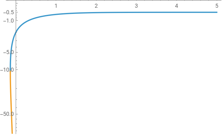
The two branches start at the same point and increase and decrease respectively. The -1 branch is defined only over a narrow range of values of L.
Plot[{qL0,qL1},{L,-(1/2)ProductLog[1/E],5},PlotRange->{-100,0},ScalingFunctions->"SignedLog"]
Out[]=
Why you should embrace the Lambert W function
Why you should embrace the Lambert W function
Your occupation is listed as "student", but I don't know if that's grade six or graduate school. :) If you might have a career in chemistry, physics, combinatorics, or other mathematical disciplines, the W function has proved very useful in many fields since attention was brought to it in 1996 in Corless, et al., http://dx.doi.org/10.1007/BF02124750. See Nick Higham's blog, https://nhigham.com/2016/08/23/corless-knuth-and-lambert-w/, for more.