Real quantum systems are not perfectly isolated; they constantly interact with their environment, causing noise, decoherence, and dissipation. In this project, I used the Wolfram Quantum Framework to model these open quantum systems with density matrices and Lindbladian dynamics. I simulated dephasing, amplitude damping, combined noise, entanglement decay, energy dissipation, and position dephasing in wave packets. These simulations show how different noise channels damage quantum information in different ways: dephasing destroys phase relationships, amplitude damping causes energy loss, and combined noise better reflects real hardware behavior. Additionally, I explored the physical applications of Lindbladian systems through modeling of interesting phenomena under Lindbladian evolution. Future work should explore even more various types of noise channels, and implement Lindbladian evolution for more advanced metrics of error correction and for noise model synthesis.
Introduction
Introduction
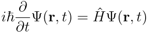
Quantum mechanics traditionally describes isolated systems through the Schrödinger equation,where the Hamiltonian generates deterministic, unitary evolution. Under this equation, a closed quantum system evolves without losing information: pure states remain pure, probabilities are conserved, and the evolution is reversible. While this idealized description provides the foundation of quantum mechanics, it assumes that the system is perfectly isolated from its surroundings.In reality, every physical quantum system interacts to some extent with its environment. These interactions continuously exchange energy and information with external degrees of freedom, causing decoherence and dissipation that cannot be accounted for by the Schrödinger equation alone. As a result, the state of the system is better represented by a density matrix ρ, whose evolution is governed by the Lindblad master equation.=[H,ρ]+ρ-{,ρ}The first term describes the familiar unitary evolution generated by the Hamiltonian (essentially just the result of rephrasing Schrödinger’s equation in terms of density matrices - this by itself called the Von Neumann equation), while the second introduces environmental interactions through a collection of Lindblad (or jump) operators . Together, these terms provide a mathematically consistent description of open quantum systems, allowing coherent dynamics and irreversible noise processes to be modeled within a single framework.
H
ρ
t
-
ℏ
∑
i
γ
i
L
i
†
L
i
1
2
†
L
i
L
i
In this computational essay, I investigated Lindbladian dynamics through a series of computational experiments using the Wolfram Quantum Framework. Rather than treating the Lindblad equation solely as a mathematical object, I used numerical simulation and visualization to build intuition for how different noise mechanisms influence quantum evolution. Beginning with the transition from closed to open systems, I progressively examined dephasing, amplitude damping, competing noise processes, and entanglement, using each investigation to better understand how Lindbladian dynamics models the behavior of realistic quantum systems, eventually tying it to real physical phenomena.
Modeling Open Quantum Systems with Lindbladian Dynamics
Modeling Open Quantum Systems with Lindbladian Dynamics
Before studying specific noise mechanisms, I first wanted to create computational picture of what Lindbladian dynamics changes about quantum evolution. In closed-system quantum mechanics, the Hamiltonian rotates the state while preserving purity. For a single qubit, this means that pure states remain on the surface of the Bloch sphere. Lindbladian dynamics adds environmental interactions to this evolution, allowing trajectories to move inward as the state becomes mixed.
Setting up Lindbladian Evolution
Setting up Lindbladian Evolution
To model Lindbladian dynamics, I used the function QuantumEvolve, providing the regular Hamiltonian as well as additional jump operators (along with their γ values that govern the rate of interference by defining the probability that they occur at a certain time). I then visualized the evolution through plotting states over time on a Bloch sphere.
Import the QuantumFramework Paclet:
In[]:=
<<Wolfram`QuantumFramework`
Define a function that evolves several initial states under a Liouvillian and displays their Bloch sphere trajectories over time:
In[]:=
simulateEvolution[jumpOperators_,gammaValues_,startingStates_,time_]:=DynamicModule[{operator,evolutions,trajectoryFunctions,colors},operator=QuantumOperator["Liouvillian"[QuantumOperator["X"],jumpOperators,gammaValues]];evolutions=Map[QuantumEvolve[Ioperator,#,{τ,0,time}]&,startingStates];trajectoryFunctions=Map[#[τ]["BlochVector"]&,evolutions];colors=ColorData["BrightBands"]/@Rescale[Range[Length[startingStates]]];With[{tf=trajectoryFunctions,cols=colors},Manipulate[Show[ResourceFunction["BlochSpherePlot"][],MapThread[ParametricPlot3D[#1,{τ,0.0001,f},PlotStyle->{#2,Thick}]&,{tf,cols}],Graphics3D[MapThread[{#2,PointSize[0.02],Point[#1/.τ->f]}&,{tf,cols}]]],{f,0.01,time,Appearance->"Labeled"},SaveDefinitions->True]]]
This function constructs a Liouvillian from two ingredients: a Hamiltonian term and a set of Lindblad jump operators. The Hamiltonian still produces motion, describing how the state would normally evolve under closed evolution, while the jump operators introduce environmental effects. Because the output is shown on the Bloch sphere, it is easy to visually separate ordinary rotation from inward contraction caused by noise.
Choose four initial qubit states and evolve them under a simple dephasing-type Lindbladian:
In[]:=
startingStates=QuantumState/@{"0","1","Plus","Minus"};
Create a jump operator
In[]:=
jumpOperators={QuantumOperator["Z"]};
Set up the simulation constants:
In[]:=
gammaValues={0.05};time=20;
Call the simulate evolution function to create a Bloch plot over time:
In[]:=
simulateEvolution[jumpOperators,gammaValues,startingStates,time]
Out[]=


The resulting trajectories do not simply rotate on the surface of the Bloch sphere. Instead, they spiral or contract inward. This inward motion is the geometric signature of open-system behavior: the state is no longer remaining pure. In density-matrix language, environmental interaction causes information about the state to leak into the surroundings, turning a pure state into a mixed state.
Comparison to a closed system
Comparison to a closed system
Then, I tried to do the same thing with a closed system: now I instead use the Schrodinger equation to model evolution over time. I then compared the visualizations to attempt to get a clearer picture of what the jump operators in the Lindblad master equation really do.
Define a comparison function that evolves the same initial states using only Schrödinger evolution, with no Lindblad jump operators:
In[]:=
simulateSchrodingerEvolution[startingStates_,time_]:=DynamicModule[{operator,evolutions,trajectoryFunctions,colors},operator=QuantumOperator["X"];evolutions=QuantumEvolve[operator,#,{τ,0,time}]&/@startingStates;trajectoryFunctions=#[τ]["BlochVector"]&/@evolutions;colors=ColorData[97]/@Range[Length[startingStates]];With[{tf=trajectoryFunctions,col=colors},Manipulate[Show[ResourceFunction["BlochSpherePlot"][],Evaluate@Table[ParametricPlot3D[Evaluate[tf[[i]]],{τ,0.0001,f},PlotStyle->{col[[i]],Thick},PlotRange->{{-1,1},{-1,1},{-1,1}}],{i,Length[tf]}],Graphics3D[Table[{col[[i]],PointSize[0.025],Point[Evaluate[tf[[i]]/.τ->f]]},{i,Length[tf]}]],PlotLabel->"Schrodinger Evolution on the Bloch Sphere",ImageSize->Medium],{f,0.01,time,AppearanceElements->{"PlayPauseButton","ProgressSlider"}},SaveDefinitions->True]]]
Call the function to simulate the same starting states over time:
In[]:=
simulateSchrodingerEvolution[startingStates,time]
Out[]=

The difference between the two visualizations is the central distinction between closed- and open-system dynamics. In contrast to the Lindbladian model, the Schrodinger evolution’s trajectories remain on the surface of the Bloch sphere. This reflects the fact that unitary evolution preserves pure states: the Hamiltonian changes the state’s direction, but not its purity (a Hamiltonian cannot make a pure state mixed).
Purity as a Comparison Metric
Purity as a Comparison Metric
For further analysis, I tracked the purity of two identical starting states over time under each system, and plotted a graph to visualize the metrics.
Use QuantumEvolve to define the closed state (time evolution governed by Schrodinger’s equation):
In[]:=
closedEvolution=QuantumEvolve[QuantumOperator["X"],QuantumState["Plus"],{τ,0,time}];
Define a Lindbladian super-operator as a collective operator to apply on the density matrix:
In[]:=
openOperator=QuantumOperator["Liouvillian"[QuantumOperator["X"],jumpOperators,gammaValues]];
Use the operator and QuantumEvolve to create Lindbladian evolution:
In[]:=
openEvolution=QuantumEvolve[IopenOperator,QuantumState["Plus"],{τ,0,time}];
Use Plot to graph purity over time for both evolutions:
In[]:=
PlotEvaluate[{closedEvolution[τ]["Purity"],openEvolution[τ]["Purity"]}],{τ,0,time},
Out[]=
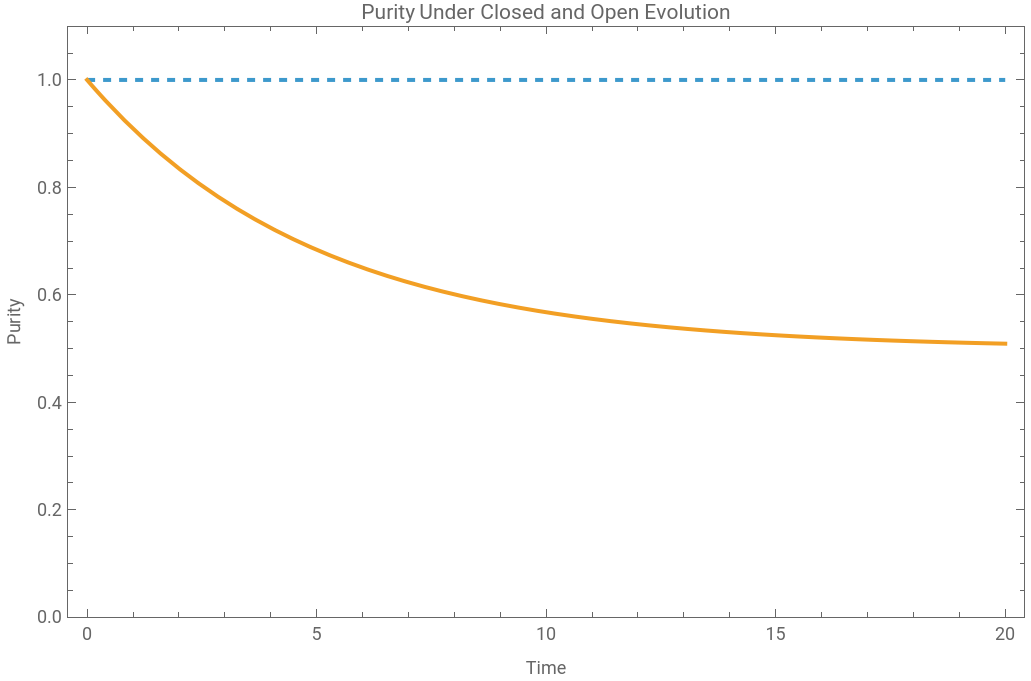


The Purity graph aligns with the same behavior seen in the Bloch sphere simulations. Under Schrödinger evolution, the purity remains equal to one, meaning the state remains pure for the entire evolution. Under Lindbladian evolution, the purity decreases over time, showing that the system is no longer fully described by a single pure state.
Dephasing, Rates and State Dependence
Dephasing, Rates and State Dependence
A quick shorthand dephasing function defined for convenience:
Now use this function to simulate as many states as needed.
Comparing Different Rates of Dephasing Over Time.
Comparing Different Rates of Dephasing Over Time.
This metric measures the magnitude of the upper off-diagonal density matrix entry ρ . It is not a full,universal measure of coherence (I often refer to it as “coherence” for the sake of simplicity), but it tracks the phase-sensitive relationship between the two basis states. As dephasing destroys that relationship, this metric should ideally decrease, because the phase relationship between both states is precisely what is being effected.
Create shorthand function to quickly get a measure of the effect of dephasing:
With a measure of dephasing defined, its possible to now test how the dephasing rate affects the evolution. The Lindblad rate γ controls the strength of the environmental interaction. If the model is behaving as expected, larger values of γ should cause the chosen coherence measure to decay more rapidly. The approach was to create multiple evolutions, each with the same initial state but different gamma values for the dephasing operator. Then, I plotted the quantum coherence (from the off-diagonal of the density matrices of the states) to see how it decreases over time for each rate.
Define an initial state:
Define a list of gamma values to test:
Create a list of evolutions for each gamma value:
Generate a list of curves showing the dephasing metric at certain points in time for the purpose of a graph:
Graph curves:
As expected, larger gamma values led to a faster decay. In fact, it is observed the time to decay to a certain level of coherence forms an inverse relationship with the gamma value: a gamma value of 0.1 took around 20 seconds to decay to a value of 0.009 on the dephasing metric, while 0.2 took only 10 seconds, and the fastest was 0.4 with 5 seconds.
Comparing Different States Dephasing Over Time.
Comparing Different States Dephasing Over Time.
The previous simulation showed that the dephasing rate controls how quickly a superposition loses it . The next question is whether this behavior depends on the initial state . Dephasing acts relative to a particular basis, so states aligned with that basis should behave differently from states that store information in phase relationships.
Choose several initial states to compare under the same dephasing channel:
Construct the corresponding quantum states:
Fix the dephasing rate and time for a proper comparison:
Create evolutions, this time for each different state:
Generate curves by taking the metric at different times:
Create a legend by numbering the random mixed states and joining them with the special states:
Plot the curves alongside the legend (plot labels):
The superposition states Plus and Minus begin with large off-diagonal density matrix entries, so their coherence decays under dephasing. In contrast, the computational basis states 0 and 1 begin with no off-diagonal coherence in this basis, so this particular coherence measure remains near zero for them.
This shows that dephasing does not affect every state in the same way. It specifically destroys phase relationships between the computational basis states. States that are already aligned with the dephasing basis (0 and 1) are comparatively stable, while states in superposition are fragile.
One can also visualize those same states on the Bloch sphere. I added a Hamiltonian (operator X) to make things a bit more intriguing geometrically. When simulating under dephasing, interesting spirals that converge inside to the center are seen.
This shows that dephasing does not affect every state in the same way. It specifically destroys phase relationships between the computational basis states. States that are already aligned with the dephasing basis (0 and 1) are comparatively stable, while states in superposition are fragile.
One can also visualize those same states on the Bloch sphere. I added a Hamiltonian (operator X) to make things a bit more intriguing geometrically. When simulating under dephasing, interesting spirals that converge inside to the center are seen.
Visualize the same state dependence geometrically on the Bloch sphere:
The Bloch sphere visualization gives a geometric interpretation of what happens under dephasing. As each state spirals around the Bloch sphere, the dephasing operator pulls it towards the z-axis, decreasing the radius of rotation for each state. This eventually brings the states toward the center of the Bloch sphere.
Comparing and Combining Noise Channels
Comparing and Combining Noise Channels
Dephasing is only one possible Lindblad noise mechanism. It mainly suppresses phase information while preserving population in the computational basis. Another important noise process is amplitude damping, which models relaxation from an excited state toward a lower-energy state. Physically, this represents energy leaving the system and entering the environment.
Comparing dephasing and amplitude damping is useful because they damage a quantum state in different ways. Dephasing destroys coherence without directly changing basis populations, while amplitude damping changes the population itself. Real quantum systems often experience both processes at once, so after comparing them separately, I combined them into a single Lindbladian model.
Comparing dephasing and amplitude damping is useful because they damage a quantum state in different ways. Dephasing destroys coherence without directly changing basis populations, while amplitude damping changes the population itself. Real quantum systems often experience both processes at once, so after comparing them separately, I combined them into a single Lindbladian model.
Comparing Coherence Over Time
Comparing Coherence Over Time
I first analyzed the dephasing metric (based on the non-diagonal density matrix elements) from earlier, but this time on different evolutions which have different combinations of noise channels to see how mixing two different types of noise can differently affect a state.
Set the initial state to Plus so that both phase coherence and population changes can be observed:
Set constants for the simulation:
Create the operators, keep the Hamiltonian blank since we’re focusing on noise:
The Pauli Z operator creates dephasing because it distinguishes the computational basis states without transferring population between them. The lowering operator J- creates amplitude damping because it models relaxation from the excited state to the lower-energy state. These two jump operators therefore represent physically different ways for the environment to affect the same qubit.
Define a dephasing only Lindblad operator:
Define an amplitude damping only Lindblad operator:
Define a operator that applies both dephasing and amplitude damping:
Create evolutions with the respective operators:
Create the curves looking at the dephasing metric over time for each evolution:
Plot the curves:
The coherence comparison shows that both dephasing and amplitude damping can reduce off-diagonal structure, but they do so for different physical reasons. Dephasing directly suppresses phase relationships, while amplitude damping changes the state by relaxing population toward a preferred energy state (the ground state). When both channels act together, coherence decays faster because the state is being affected by two independent environmental mechanisms. However, it is clearly evident that dephasing does much more of the work here, aligning with the fact that it directly decays the off diagonal elements to 0.
Comparing Purity Over Time
Comparing Purity Over Time
I can also show the purity over time for each noise channel. Purity measures how “pure” or unmixed a quantum state is, using the trace of the square of the density matrix. In this comparison, purity shows how fast noise channel is turning the state from a definite superposition to a mixture of states, which can geometrically be thought as how the Bloch vector norm (length) decreases over time.
Sample purity over time for the three noise models:
Plot the purity curves over time for all three noise possibilities:
Purity gives a different perspective from coherence, and a much more interesting one . Dephasing turns a pure superposition into a mixed state by destroying phase information . Amplitude damping can also reduce purity, but its long - term behavior is different because it pushes the system toward a particular final state rather than simply erasing phase. The graph aligns with physical predictions. This is because amplitude damping always sends a state towards the ground or zero state as time progresses, which geometrically corresponds to the north pole of the Bloch sphere. Since the ground state is a pure state itself, both Lindbladian evolutions that have amplitude damping level off at a purity of 1. Since the initial state of plus has an equal distribution of 0 and 1, dephasing causes it to become a complete classical 50-50 mixture of the two states, meaning it lies at the origin of the Bloch sphere, and thus has no purity.
Comparing Probabilities/Populations Over Time
Comparing Probabilities/Populations Over Time
I also looked at the excited state (|1〉 in braket notation) over time for each of these states . This particularly is useful for qubit/quantum systems where the property of energy is being considered, such as the energy of an electron .
Define the excited-state population as the second diagonal entry of the density matrix:
Sample the excited-state population for each noise model:
Plot the excited-state population under the three noise models:
The population plot reveals the clearest physical difference between the two noise channels . Dephasing leaves the excited - state population essentially unchanged, because it acts on phase rather than energy . Amplitude damping reduces the excited - state population because it models relaxation toward the lower - energy state.
The combined channel inherits both behaviors : it loses coherence while also relaxing population . This is the main reason amplitude damping and dephasing, as well as other noise channels, cannot be treated as interchangeable forms of "noise ." They affect different parts of the density matrix and represent different physical interactions with the environment. Since dephasing does not affect probabilities themselves, the line remains flat at 0.5. However, because amplitude damping moves everything to the low/ground energy state, the probability of being at the excited state goes to 0.
The combined channel inherits both behaviors : it loses coherence while also relaxing population . This is the main reason amplitude damping and dephasing, as well as other noise channels, cannot be treated as interchangeable forms of "noise ." They affect different parts of the density matrix and represent different physical interactions with the environment. Since dephasing does not affect probabilities themselves, the line remains flat at 0.5. However, because amplitude damping moves everything to the low/ground energy state, the probability of being at the excited state goes to 0.
Entanglement, Noise Sensitivity and Noise-Resistant States
Entanglement, Noise Sensitivity and Noise-Resistant States
The previous sections focused mostly on single-qubit noise. However, useful quantum systems are usually multi-qubit systems, and many important quantum states store information in correlations between qubits. This makes multi-qubit Lindbladian evolution especially important.
In a multi-qubit system, the jump operators can represent different physical noise structures. Noise can act independently on each qubit, or it can act in a correlated way on multiple qubits at once. These two cases can produce very different behavior, even when the noise mechanism is still dephasing.
In a multi-qubit system, the jump operators can represent different physical noise structures. Noise can act independently on each qubit, or it can act in a correlated way on multiple qubits at once. These two cases can produce very different behavior, even when the noise mechanism is still dephasing.
Independent vs. Correlated Dephasing
Independent vs. Correlated Dephasing
In this section, I first compared independent and correlated dephasing on a Bell state . Then, I compared several important three - qubit states under different noise channels to identify which states are more noise - resistant. This can help conceptually understand the difference between these two seemingly similar types of dephasing.
Create a dephasing operator acting only on the first qubit:
Create a dephasing operator acting only on the second qubit :
Create a correlated dephasing operator acting on both qubits together:
Set the constants for evolution:
Construct the independent dephasing Liouvillian:
Construct the correlated dephasing Liouvillian:
Define the Bell state used to compare the two noise models:
Evolve the Bell state under independent dephasing:
Evolve the Bell state under correlated dephasing:
To measure the entanglement of the Bell state over time, I used concurrence (using the non-diagonal density matrix elements) . Concurrence is useful here because the Bell state is a two - qubit state, and concurrence directly tracks how much two - qubit entanglement remains during the evolution .
Sample Bell-state concurrence under independent and correlated dephasing:
Plot the Bell-state entanglement under the two dephasing models:
This graph shows that the structure of the noise matters. Independent dephasing acts separately on the two qubits, so it can destroy the phase relationship that supports Bell-state entanglement. Correlated dephasing acts differently because the environment couples to the joint two-qubit structure
For this Bell state, correlated dephasing can be less damaging (actually not damaging at all) because the two components of the Bell state are affected in a more symmetric way. In contrast, the independent dephasing caused a decay in concurrence, as the phase relationship that was originally there between the qubits is destroyed via dephasing.This introduces an important idea: a state can be fragile under one noise model but resistant under another. Noise resistance is not just a property of the state by itself; it depends on the relationship between the state and the Lindblad operators.
For this Bell state, correlated dephasing can be less damaging (actually not damaging at all) because the two components of the Bell state are affected in a more symmetric way. In contrast, the independent dephasing caused a decay in concurrence, as the phase relationship that was originally there between the qubits is destroyed via dephasing.This introduces an important idea: a state can be fragile under one noise model but resistant under another. Noise resistance is not just a property of the state by itself; it depends on the relationship between the state and the Lindblad operators.
GHZ and W States
GHZ and W States
I now extended the analysis to three - qubit states . Two especially important examples are the GHZ state and the W state . The GHZ state is a superposition of all qubits being 0 and all qubits being 1. The W state is a superposition of one excitation being shared across three qubits . These states are both entangled, but they store their quantum information differently . Because of that, they may respond differently to dephasing and amplitude damping . I also included the |000〉 state and the |+++〉 state as reference states . The |000〉 state should be stable against dephasing because it has no off - diagonal phase structure, while |+++〉 is a highly coherent product state .
Set the number of qubits for the state comparison experiment:
Construct independent three-qubit dephasing operators:
Define the lowering matrix for amplitude damping:
Construct independent three-qubit amplitude damping operators:
The three-qubit dephasing operators apply local phase noise to each qubit. The amplitude damping operators apply local relaxation noise to each qubit. This creates a comparison between two different physical mechanisms acting on the same set of initial states.
Define the three-qubit GHZ state:
Define the three-qubit W state:
Define the three-qubit |+++〉 state:
Define the three-qubit |000〉 state:
Store the states and labels together.
These four states give a useful range of behavior. GHZ and W are both entangled but structurally different. The +++ state is not entangled, but it contains a large amount of single-qubit coherence. The 000 state is a computational-basis state, so it should be resistant to dephasing however the drawback being that this state contains little useful information.
Fidelity over Time for Different States
Fidelity over Time for Different States
I also tracked another metric called fidelity. Fidelity measures the closeness of a state after evolution to what it should ideally by computing the trace of the product of both density matrices. I then analyzed and compared different states’ fidelities over time to conclude which states are prone and which states are immune to certain types of quantum noise.
Set the rate and time interval for the three-qubit comparison:
Construct the three-qubit independent dephasing Liouvillian:
Construct the three - qubit independent amplitude damping Liouvillian:
For three-qubit states, concurrence is no longer the best metric because concurrence is designed for two-qubit entanglement. Instead, I used survival fidelity: how much the evolved state still overlaps with the initial state. This gives a direct way to compare noise resistance across GHZ, W, |+++〉, and |000〉. A state with higher fidelity over time is more resistant to that noise channel.
Evolve each comparison state under three-qubit dephasing:
Sample survival fidelity under dephasing:
Plot the noise resistance of the comparison states under dephasing:
The dephasing fidelity plot shows which states preserve their original structure most effectively. The |000〉 state should remain highly stable because dephasing does not change computational-basis populations. The |+++〉 state is more vulnerable because it stores information in phase coherence. The GHZ and W states are both entangled, but they can decay at different rates because their coherence is distributed across different basis components, with the W state’s fidelity unaffected and the GHZ’s fidelity decreasing over time.
Evolve each comparison state under three-qubit amplitude damping:
Sample survival fidelity under amplitude damping:
Plot the noise resistance of the comparison states under amplitude damping:
The amplitude damping plot gives a different ranking from the dephasing plot. This is expected because amplitude damping changes energy population rather than only suppressing phase. States with excitations are vulnerable because amplitude damping relaxes those excitations toward the ground state. The |000〉 state is especially stable under amplitude damping because it is already the relaxed state.
The W state and GHZ state respond differently because their excitations are arranged differently. The W state contains one excitation spread across the system, while the GHZ state includes a component where all three qubits are excited. It is observed that the W state is completely unaffected by amplitude damping in this case, and this aligns with how it is realistically resilient to amplitude damping.
The W state and GHZ state respond differently because their excitations are arranged differently. The W state contains one excitation spread across the system, while the GHZ state includes a component where all three qubits are excited. It is observed that the W state is completely unaffected by amplitude damping in this case, and this aligns with how it is realistically resilient to amplitude damping.
Define total off-diagonal coherence for a density matrix:
Sample total coherence under dephasing:
Plot total coherence under dephasing:
The total coherence, a metric totaling the off diagonal entries of the matrix, plot directly shows what dephasing removes : off-diagonal density matrix structure . States with large off - diagonal structure (phase relationship between basis states, such as |+++〉 lose coherence over time, while basis states have little or no off |000〉 - diagonal structure lose less under the same Lindbladian dephasing channel. The W state is robust to this type of dephasing, because it acts as an eigenstate to this jump operator.
Physical Applications of Lindbladian Dynamics and Noise
Physical Applications of Lindbladian Dynamics and Noise
The earlier sections treated Lindblad operators mainly as abstract noise models. In this section, I connect those same mathematical tools to simple physical systems. I did this by showing how realistic Hamiltonians and Lindblad jump operators can work together to model physical open-system behavior.
Energy Dissipation
Energy Dissipation
I used scaled units where ℏ (reduced Planck’s constant) =1. This means frequencies, energies, and decay rates are written in compatible dimensionless units. The Hamiltonian describes the system’s internal physical evolution, while the Lindblad operators describe how the environment modifies that evolution.
Construct the two-level Hamiltonian:
Use the lowering operator as the amplitude damping jump operator:
Choose a relaxation rate and simulation time:
Construct the Lindbladian for energy relaxation:
Start the system in the excited state:
Evolve the excited state under the relaxation Lindbladian, and display the symbolic equation:
Now that I have an equation in terms of time to represent the energy state over time, I took a limit to see what happens in the long run (when time goes to infinity)
Take the limit as time goes to infinite of the evolution:
The limit approaches the state vector {1, 0}, meaning the probability the energy level is at ground (lowest) level is 1. This makes sense: since no additional energy is being added to the environment, an amplitude damping is the only thing acting on the system, the energy is bound to be completely dissipated. Additionally, the dissipation can be modeled as exponential decay of the high energy state, giving an insight as to how electrons lose their energy when moving back to the ground state in an atom.
Wave Packets and Dephasing
Wave Packets and Dephasing
A more physical version of the two-path model is a wave packet spread across many position states. Instead of representing only “path 1” and “path 2,” I represented a particle or spin packet on a one-dimensional lattice of possible positions. The state vector now stores an amplitude at each position.
In this model, I approximated continuous space by looking at it as a finite, discrete set of position sites. Each site acts like a basis state of the quantum system, so the wave packet is represented as a quantum state spread across these possible positions. This allows one to study position-based dephasing by tracking how the density matrix evolves between different spatial sites.
In this model, I approximated continuous space by looking at it as a finite, discrete set of position sites. Each site acts like a basis state of the quantum system, so the wave packet is represented as a quantum state spread across these possible positions. This allows one to study position-based dephasing by tracking how the density matrix evolves between different spatial sites.
Set up a one-dimensional position lattice:
Define a Gaussian wave packet on the position lattice:
Create an initial wave packet localized slightly to the left:
Visualize the discretization and initial Gaussian distribution of the wave packet:
The Gaussian envelope makes the state localized in space, while the complex phase factor gives the packet a momentum-like direction. This is still a simplified lattice model, but it is much closer to a wave packet than a two-state path model.
Set the hopping strength and position-dependent gradient strength:
Build the tight-binding Hamiltonian matrix.
Convert the Hamiltonian matrix into a quantum operator.
The off-diagonal entries of the Hamiltonian let amplitude move between neighboring sites, creating wave-packet spreading. The diagonal gradient term gives different positions different energies, causing position-dependent phase evolution. This resembles the way spatially varying magnetic fields create phase differences across an MRI sample.
Define projection operators onto each position state:
Set the spatial dephasing rate and simulation time:
Construct the Lindbladian for position-basis dephasing:
Each position projector acts like an environmental interaction that partially measures where the packet is. The environment does not need to fully collapse the state at once. Instead, the Lindblad evolution gradually suppresses coherence between different positions. This is the density-matrix version of losing a well-defined phase relationship across the packet.
Evolve the wave packet with position - basis dephasing:
Define the position probability distribution from the density matrix:
Define a list of times to sample the distribution at:
I then tried to create a visualization to show how the state evolves over time via a manipulate that changes time, which causes the distribution of the probabilities to change on the graph as the density matrix changes under Lindbladian evolution. Additionally, I used the non-diagonal elements of the matrix, which represents two-wise products between different states, to get their phase relationship. Since the phase cannot be visualized as a dimension on this graph, I gave it a certain color on a scale of -π to π.
Create a function to get the relative phases at all positions in the density matrix:
Create a list of the relative phases of the wave at certain points in time:
Create a function to map each phase to a certain color of the rainbow:
Create a few slices per interval to help the wave look smoother:
Find the maximum probability any state achieves across all times to help rescale y-values:
Create a function that plots the wave distribution with phase coloring over time:
Call the function through a manipulate that allows one to see the wave packet,distribution change as a function of time:
At t=0, the wave packet starts as a localized Gaussian-like distribution centered near the left side of the position grid. As time evolves, the Hamiltonian causes the packet to spread and move across the discretized position sites, while the position dephasing noise disrupts the phase relationships between neighboring sites. This is why the packet gradually loses its clean wave-like shape and becomes more spread out and flattened over time.
Physically, this can be understood with the example of a photon whose position-state is being disturbed by environmental noise. The environment is not necessarily “measuring” the photon directly, but potential interactions (via dephasing) gives partial information about where the photon could be, which weakens the phase relationships needed for interference. As a result, the photon’s state becomes less like a clean coherent wave packet and more like a mixed distribution over many possible positions.
The colored regions show the local phase relationships between neighboring position sites. Early on, the phase structure is more organized, but as dephasing progresses, those relationships become disrupted, and then become similar when the distribution relaxes near the end.
Physically, this can be understood with the example of a photon whose position-state is being disturbed by environmental noise. The environment is not necessarily “measuring” the photon directly, but potential interactions (via dephasing) gives partial information about where the photon could be, which weakens the phase relationships needed for interference. As a result, the photon’s state becomes less like a clean coherent wave packet and more like a mixed distribution over many possible positions.
The colored regions show the local phase relationships between neighboring position sites. Early on, the phase structure is more organized, but as dephasing progresses, those relationships become disrupted, and then become similar when the distribution relaxes near the end.
Conclusion
Conclusion
Real quantum systems are never perfectly isolated. Because they exchange energy and information with their environment, their evolution cannot always be described by the Schrödinger equation alone. Instead, density matrices and the Lindblad master equation provide a more realistic framework for modeling quantum systems by including the error and noise they experience due to external effects.
I first found that dephasing destroys a superposition by suppressing the off-diagonal density-matrix terms, and that larger values of γ produce faster decay. The starting state also matters: states aligned with the noise basis are much more stable, while superposition states are more vulnerable because their information depends on phase relationships between basis states.
I then compared dephasing with amplitude damping and found that they represent physically different types of noise. Dephasing mainly destroys phase information while leaving populations mostly unchanged, while amplitude damping transfers population from the excited state to the ground state, representing energy loss. When both channels act simultaneously, the state loses both phase coherence and excitation, which is closer to the behavior of real qubits, where all types of noise can act.
The entanglement simulations showed that entangled states can be especially sensitive to noise, because their information is stored in correlations across multiple qubits rather than in one isolated state. However, the simulations also showed that some states can be naturally resistant to specific noise channels, such as how the GHZ state is resistant against dephasing and how the W state is resistant to amplitude damping. This is an important idea behind error correction: instead of fighting every error directly, encode information into states or subspaces where the most likely errors have reduced effect.
The physical applications extended these ideas beyond abstract qubits. In the energy dissipation simulation, amplitude damping caused an excited system to lose energy and relax toward the ground state, showing how Lindblad dynamics can model irreversible decay. In the wave-packet simulation, position dephasing disrupted the phase relationships across different spatial sites, causing the packet to go through a disruptive motion before collapsing into a relaxed state.
I first found that dephasing destroys a superposition by suppressing the off-diagonal density-matrix terms, and that larger values of γ produce faster decay. The starting state also matters: states aligned with the noise basis are much more stable, while superposition states are more vulnerable because their information depends on phase relationships between basis states.
I then compared dephasing with amplitude damping and found that they represent physically different types of noise. Dephasing mainly destroys phase information while leaving populations mostly unchanged, while amplitude damping transfers population from the excited state to the ground state, representing energy loss. When both channels act simultaneously, the state loses both phase coherence and excitation, which is closer to the behavior of real qubits, where all types of noise can act.
The entanglement simulations showed that entangled states can be especially sensitive to noise, because their information is stored in correlations across multiple qubits rather than in one isolated state. However, the simulations also showed that some states can be naturally resistant to specific noise channels, such as how the GHZ state is resistant against dephasing and how the W state is resistant to amplitude damping. This is an important idea behind error correction: instead of fighting every error directly, encode information into states or subspaces where the most likely errors have reduced effect.
The physical applications extended these ideas beyond abstract qubits. In the energy dissipation simulation, amplitude damping caused an excited system to lose energy and relax toward the ground state, showing how Lindblad dynamics can model irreversible decay. In the wave-packet simulation, position dephasing disrupted the phase relationships across different spatial sites, causing the packet to go through a disruptive motion before collapsing into a relaxed state.
Limitations & Future Directions
Limitations & Future Directions
My study of Lindbladian dynamics has many limitations for the sake of simplicity and achievability. One limitation is that I focused mainly on dephasing and amplitude damping, even though real quantum hardware can also experience coherent drift, crosstalk, leakage, correlated noise, heating, and gate-dependent noise. I also used mostly abstract or normalized parameter values rather than precise device-calibrated values, so the simulations show qualitative behavior rather than making exact predictions for a specific machine.
Another limitation is that most of the project studies small systems and isolated noise effects. This made it possible to clearly see how each noise channel changes coherence, purity, population, entanglement, and spatial phase structure. However, real quantum devices involve many interacting qubits, gates, measurements, and hardware-specific timescales. Future versions of this work could use experimentally motivated parameters, larger Hilbert spaces, and more realistic multi-qubit noise models.
One natural future direction is to incorporate a wider variety of Lindblad noise channels. This could include coherent Z-drift, ZZ crosstalk, correlated dephasing, leakage-like effects, thermal excitation, or noise operators fitted to real hardware. This would make the simulations even closer to those that can be used to model realistic, practical systems.
A second direction is to use Lindblad dynamics to test quantum error correction more realistically. Standard error-correction analysis often assumes discrete Pauli errors such as bit flips and phase flips, but Lindblad evolution can represent continuous physical noise before it is simplified into a Pauli model. Recent work studies exactly this issue: how error-correction success changes when the code is exposed to physically motivated Lindblad noise rather than only idealized Pauli errors. This suggests that future simulations could encode logical states, evolve them under a Liouvillian, apply syndrome correction, and compare how well different codes protect information.
A third and more advanced direction is Lindblad noise synthesis. In this context, synthesis means starting from a physical Lindbladian, or a learned Lindbladian from hardware data, and constructing the effective noise channel that a gate or circuit actually experiences. This is important because the same underlying physical noise can appear differently depending on the gate being applied. A future direction could include exploring how this works in the Wolfram Quantum Framework and what noise synthesis can be applied.
Another limitation is that most of the project studies small systems and isolated noise effects. This made it possible to clearly see how each noise channel changes coherence, purity, population, entanglement, and spatial phase structure. However, real quantum devices involve many interacting qubits, gates, measurements, and hardware-specific timescales. Future versions of this work could use experimentally motivated parameters, larger Hilbert spaces, and more realistic multi-qubit noise models.
One natural future direction is to incorporate a wider variety of Lindblad noise channels. This could include coherent Z-drift, ZZ crosstalk, correlated dephasing, leakage-like effects, thermal excitation, or noise operators fitted to real hardware. This would make the simulations even closer to those that can be used to model realistic, practical systems.
A second direction is to use Lindblad dynamics to test quantum error correction more realistically. Standard error-correction analysis often assumes discrete Pauli errors such as bit flips and phase flips, but Lindblad evolution can represent continuous physical noise before it is simplified into a Pauli model. Recent work studies exactly this issue: how error-correction success changes when the code is exposed to physically motivated Lindblad noise rather than only idealized Pauli errors. This suggests that future simulations could encode logical states, evolve them under a Liouvillian, apply syndrome correction, and compare how well different codes protect information.
A third and more advanced direction is Lindblad noise synthesis. In this context, synthesis means starting from a physical Lindbladian, or a learned Lindbladian from hardware data, and constructing the effective noise channel that a gate or circuit actually experiences. This is important because the same underlying physical noise can appear differently depending on the gate being applied. A future direction could include exploring how this works in the Wolfram Quantum Framework and what noise synthesis can be applied.
References
References
Amplitude damping channel. (n.d.). In Wikipedia. Retrieved July 9, 2026, from https://en.wikipedia.org/wiki/Amplitude_damping_channel
Brasil, C. A., Fanchini, F. F., & Napolitano, R. de J. (2012). A simple derivation of the Lindblad equation. arXiv. https://arxiv.org/abs/1110.2122
Coherence (physics). (n.d.). In Wikipedia. Retrieved July 9, 2026, from https://en.wikipedia.org/wiki/Coherence_(physics)
Dephasing. (n.d.). In Wikipedia. Retrieved July 9, 2026, from https://en.wikipedia.org/wiki/Dephasing
Lindbladian. (n.d.). In Wikipedia. Retrieved July 9, 2026, from https://en.wikipedia.org/wiki/Lindbladian
Malekakhlagh, M., Seif, A., Puzzuoli, D., Govia, L. C. G., & van den Berg, E. (2025). Efficient Lindblad synthesis for noise model construction. npj Quantum Information, 11, Article 191. https://doi.org/10.1038/s41534-025-01139-1
Manzano, D. (2020). A short introduction to the Lindblad master equation. AIP Advances, 10(2), 025106. https://doi.org/10.1063/1.5115323
Schrödinger equation. (n.d.). In Wikipedia. Retrieved July 9, 2026, from https://en.wikipedia.org/wiki/Schr%C3%B6dinger_equation
Schrodinger Equation Simulator. (n.d.). Retrieved July 9, 2026, from https://schrodingerequation.online/
Schwartzman-Nowik, Z., Shirizly, L., & Landa, H. (2025). Modeling error correction with Lindblad dynamics and approximate channels. Physical Review A, 111(2), 022613. https://doi.org/10.1103/PhysRevA.111.022613
Wave packet. (n.d.). In Wikipedia. Retrieved July 9, 2026, from https://en.wikipedia.org/wiki/Wave_packet#Gaussian_wave_packets_in_quantum_mechanics
Acknowledgements
Acknowledgements
I would like to sincerely thank my mentor Bruno Tenorio for all the guidance and expertise he provided. This is my first rigorous study of a quantum mechanics topic, and it would have been nowhere near possible without his help with explaining the concepts, helping me figure out my code, and shaping the structure and direction of my essay.
Additional thanks to Stephen Wolfram for suggesting this project. The idea of exploring Lindbladian dynamics using Wolfram Mathematica, as well as the idea of representing Lindbladian evolution using a wave packet form, which ultimately led to a beautiful visualization. I would also like to thank all the other mentors, TAs and staff who provided me support along the way, especially Daniel Xu for his support during my time here at WSRP. Lastly, I would like to express my gratitude for all the people whom I have met here and the directors for the wonderful opportunity to meet and learn from everyone at the program: this experience has been one of the most memorable and enjoyable periods of my life.
CITE THIS NOTEBOOK
CITE THIS NOTEBOOK
Modeling quantum noise channels using Lindbladian dynamics
by Samarth Sharma
Wolfram Community, STAFF PICKS, July 9, 2026
https://community.wolfram.com/groups/-/m/t/3751239
by Samarth Sharma
Wolfram Community, STAFF PICKS, July 9, 2026
https://community.wolfram.com/groups/-/m/t/3751239