ABSTRACT (original article): The rotating equilibrium solutions of 𝑁 identical point vortices are the stationary energy states of a higher-dimensional object projected to the 𝑥−𝑦 plane, in this case, an (𝑁−1)-dimensional regular simplex. Parameterizing the point vortex Hamiltonian with this fundamental geometrical object leads to a simple bivector condition, which contains the equilibrium states and resolves the origin of the asymmetric solutions. This novel approach uses the geometric product and the multivector derivative, , of the Hamiltonian in the geometric algebra, 𝐶𝑙(𝑁−1,0) to find a geometric condition that determines the equilibrium states. The resulting bivector equation is then used as the input to an optimizer, which rotates a simplex until the equilibrium condition is met, leading to a wealth of new solutions. If the vertices of the oriented simplex are projected to the 𝑥-axis, the values form the roots of the Hermite polynomials, (𝑥), and obey the Stieltjes relations, capturing the collinear solutions. The vortex simplex exhibits a striking geometrical connection with the amplituhedron of quantum field theory and gives deep insight into the quantization of a classical system. CITATION (original article): Robertson Phillip (2024), A general solution for rotating lattices of identical point vortices. Proc. R. Soc. A. 480: 20230237. http://doi.org/10.1098/rspa.2023.0237
𝜕
𝜓
𝐻
N
Introduction
Introduction
Point vortices are deceptively simple objects which capture vorticity in an ideal fluid in two dimensions. In this sense, point vortices are like little tornadoes in that they possess only ‘spin’, as opposed to coulomb force particles which either attract or repel according to an inverse square law, like massive particles for gravity and charged particles for electromagnetism. Originally invented by Helmholtz in the 19th century, point vortices experienced a resurgence of interest following the discovery of quantized vortices in liquid Helium, and in fact, they occur elsewhere in nature! Bose-einstein condensates and Type II superconductors all exhibit quantized vortices. They are even thought to occur in neutron stars because they have superfluid cores. Point vortex crystals therefore lead us directly to certain interesting quantum phenomena. A vortex crystal here means a collection of point vortices which rotate together without changing their relative distances, they rotate as if they are part of a rigid object.
These notebook figures were created for a paper, “A general solution for rotating lattices of identical point vortices,” which describes how vortex crystals are formed in this very simple model, the solution to an open problem in mathematical physics. It turns out that point vortex crystals are mysterious because they form not only radially symmetric patterns, but patterns with not symmetry at all. This flies in the face of intuition which suggests that the crystals should all have some radial symmetry from their ‘spin’ force. The motivating question is, where does this unexpected asymmetric quality come from? The answer is that the solutions are the projections of the vertices of a generalized tetrahedron, or simplex, to a 2-dimensional plane, so that they minimize energy. Not all projections are allowed, just these special ones. Recall that a 2-d simplex is a triangle, a 3-d simplex is a tetrahedron and so on, up the dimensional ladder. So, the solutions are higher dimensional creatures, projected down to an unbounded flat world, where they all rotate together. Penrose tilings get their aperiodicity from higher dimensions as well, a type of tiling known to the mathematicians of ancient Iran.
In this notebook you can find examples of point vortex crystal solutions which are the projections of corresponding simplices.
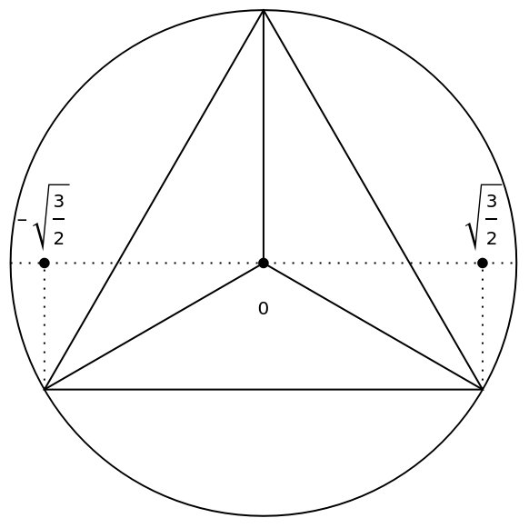
A simple vortex crystal - A triangle which projects to the roots of the Hermite polynomial
A simple vortex crystal - A triangle which projects to the roots of the Hermite polynomial
A linear vortex crystal will always have vortices which lie on the roots of a Hermite polynomial. See the paper for the supporting mathematics. It gets more interesting when the crystals are not linear.
<<"clifford.m"M=3;r=(M-1)/Sqrt[2];p1={0,r};p2={r*Cos[Pi/6],-r*Sin[Pi/6]};p3={-r*Cos[Pi/6],-r*Sin[Pi/6]};tri1={p1,p2,p3};circle1=Circle[{0,0},r];Graphics[{circle1,EdgeForm[Black],White,Triangle[tri1],Black,Line[{{0,0},p2}],Line[{{0,0},p3}],Line[{{0,0},{0,r}}],Dotted,Line[{{-r,0},{r,0}}],Line[{p2,{r*Cos[Pi/6],0}}],Line[{p3,{-r*Cos[Pi/6],0}}],PointSize[0.02],Point[{0,0}],Text[r*Cos[Pi/6],Offset[{0,25},{r*Cos[Pi/6],0}]],Point[{r*Cos[Pi/6],0}],Text[-r*Cos[Pi/6],Offset[{0,25},{-r*Cos[Pi/6],0}]],Point[{-r*Cos[Pi/6],0}],Text[0,Offset[{0,-25},{0,0}]]}]
Out[]=
Another simple vortex crystal: A tetrahedron projected to the roots of the Hermite polynomial
Another simple vortex crystal: A tetrahedron projected to the roots of the Hermite polynomial
r2=(M2-1)/Sqrt[2];s2=Sphere[{0,0,0},r2];e1={1,0,0};e2={0,1,0};p21=-+,-Sqrt[3/2],--;proj1=Projection[p21,e1];p22=+,-Sqrt[3/2],-;proj2=Projection[p22,e1];p23=--,Sqrt[3/2],+;proj3=Projection[p23,e1];p24=-,Sqrt[3/2],-+;proj4=Projection[p24,e1];
3
2
3
2
3
2
3
2
3
2
3
2
3
2
3
2
3
2
3
2
3
2
3
2
3
2
3
2
3
2
3
2
In[]:=
tet=Graphics3D[{Opacity[0.09],s2,Opacity[0.4],Tetrahedron[{p21,p22,p23,p24}],Opacity[0.5],Line[{{-r2,0,0},{r2,0,0}}],Black,Line[{p21,proj1}],Line[{p22,proj2}],Line[{p23,proj3}],Line[{p24,proj4}],PointSize[0.015],Point[proj1],Point[proj2],Point[proj3],Point[proj4],Opacity[1.0]},BoxedFalse]
Out[]=

In[]:=
hermite=ListPointPlot3D[Table[{i,0.06*HermiteH[4,i],0},{i,-1.8,1.8,0.001}]];
In[]:=
Show[tet,hermite]
Out[]=

A linear vortex crystal formed by the projection of a 5-simplex or a pentachoron to the roots of a Hermite polynomial
A linear vortex crystal formed by the projection of a 5-simplex or a pentachoron to the roots of a Hermite polynomial
In[]:=
M3=4;
In[]:=
r3=(M3-1)/2;s3=Sphere[{0,0,0},r3];sc=1/Sqrt[2];
In[]:=
Solve[HermiteH[5,x]0,x]
Out[]=
{x0},x-+,x+,x-(5-,x(5-
5
2
5
2
5
2
5
2
1
2
10
)1
2
10
)In[]:=
pentachoron=0,0,0,2+,-,-+,--5+,-,-10+,-,--,-5+;
2
,5
2
5
2
5-
,0,-5
2
1
2
5
2
5
2
1
18
2
+25
10-
,10
1
6
10
+15
10+
,-6
+10
+215
1
2
5
2
5
2
1
18
10-
-510
2
+3
-5
+30
,-1
3
5
2
6
+10
+215
1
2
5
2
5
2
1
18
10-
510
2
+3
+5
+30
,-1
6
15
10+
,-6
+10
+215
1
2
In[]:=
a1={0,0,0};a2=+,-+,--5+-,-10+;pa4=Projection[a4,e1];a5=--,-5+
5
2
5
2
5-
,0;pa2=Projection[a2,e1];a3=-5
2
5
2
5
2
1
18
2
+25
10-
,10
1
6
10
+15
10+
;pa3=Projection[a3,e1];a4=6
+10
+215
5
2
5
2
1
18
10-
-510
2
+3
-5
+30
,-1
3
5
2
6
+10
+215
5
2
5
2
1
18
10-
510
2
+3
+5
+30
,-1
6
15
10+
;pa5=Projection[a5,e1];R=DelaunayMesh[{a1,a2,a3,a4,a5}];M4=5;r4=Sqrt[15/2];s4=Sphere[{0,0,0},r4];h1=Graphics3D[{Opacity[0.06],s4,HighlightMesh[R,{Style[0,Directive[PointSize[Medium],Black]],Style[2,Opacity[0.2]]}],Opacity[0.8],Black,Line[{{-r4,0,0},{r4,0,0}}],PointSize[0.015],Point[a1],Point[pa2],Point[pa3],Point[pa4],Point[pa5],Line[{pa2,a2}],Line[{pa3,a3}],Line[{pa4,a4}],Line[{pa5,a5}]},Boxed->False]6
+10
+215
2 vortex crystals formed by the projection of the tetrahedron to the plane
2 vortex crystals formed by the projection of the tetrahedron to the plane
The first crystal below is a centered triangle.
This second crystal is a square.
A six vortex crystal projected from a 7-simplex
A six vortex crystal projected from a 7-simplex
The code below takes a list of vortex positions found by the vortex solver code, a python shell written to explore and search for point vortex solutions. The function defined below calculates the strength of the flow field for the vortex crystal at a point (x,y) in the plane.
This contour plot shows the isosurfaces for the 6 vortex system
Here is an example of a crystal formed by nine vortices projected from a 10-simplex. The values for the coordinates were found by the solver program accompanying the paper.
CITE THIS NOTEBOOK
CITE THIS NOTEBOOK
A general solution for rotating lattices of identical point vortices
by Phillip Robertson
Wolfram Community, STAFF PICKS, November 18, 2024
https://community.wolfram.com/groups/-/m/t/3323529
by Phillip Robertson
Wolfram Community, STAFF PICKS, November 18, 2024
https://community.wolfram.com/groups/-/m/t/3323529