ABSTRACT (original article): We prove that wave fronts on a flat torus become dense. As a corollary, wave fronts become dense for a square billiard or for the geodesic flow on the flat Klein bottle or the cube surface. CITATION (original article): Emily Kang, Oliver Knill, Density of wave fronts, arXiv:2501.14611. https://doi.org/10.48550/arXiv.2501.14611
Given a compact Riemannian manifold (M,g) with or without boundary, we have a global geodesic flow assuming billiard reflection at the boundary. This is all well defined if the Riemannian metric is defined except at a codimension two sets which is a union of codimension 2 manifolds. We can so for example evolve wave fronts on a polyhedron like a cube or look at a billiard in a polygonal table. If we start light at a point p, what happens with the wave front W(t) over time? Does it become dense in the manifold in the sense that for every radius r larger than 0 there exists a t(r) such that W(t) intersects every ball B(r,q) in the manifold if t is larger than t(r)? On a perfect sphere or if p is at the center of a circular pond, this does not happen, but such cases appear to be exceptional. This density problems of wave fronts seems never have been studied. There are related problems in differential geometry called “wiederkehr manifold questions” or “illumination problems”. In Summer of 2024, I worked with Harvard Undergraduate student Emily Kang on the problem of the cube. After trying almost all summer using the theory of geometry of numbers, we eventually saw a simple calculus proof [1]. One can first prove the result for flat tori. This then allows by projection to derive the results for the square or the Klein bottle or the cube. Note however that even in the flat case, we for example have no idea whether the wave fronts become dense on a regular dodecahedron. We are sure they do, but we can not prove it yet. For non-flat manifolds, definitely completely new methods might be required, maybe some larger artillery from analysis and geometry. But there could also be an easy way. We just do not know. Most of the questions one can ask appear exciting. The animations seen in [2] were made using the here included Mathematica code.
The cube
The cube
In multivariable calculus courses, we have for more than a decade asked billiard type questions like how long a path is between two points if the billiard ball has to do a certain amount of bounces on given walls. The most elegant solution is to unwrap the table. We have also asked this on a cube. Given two points on a cube what is the distance between them if you count the shortest connection on the cube as the geodesic. This can be tricky without unwrapping the cube. It was natural then to look at the problem how “circles” look like on a cube, meaning points with a given distance to a point. For larger radii, the shapes are complicated. I illustrated the problem in countless many intro lectures in multi-variable calculus courses, also just to illustrate how easy it can be to get to unsolved problems in mathematics. I wrote in 2011 the following Mathematica program, which allowed to visualize the wave fronts on a cube.
In[]:=
Out[]=

The Torus
The Torus
Here is the code for the torus, which is simpler as we just need to map the circle into the fundamental domain of the quotient R^2/Z^2.
In[]:=
ClearAll[s];r={(3+0.99*Cos[u])Cos[v],(3+0.99*Cos[u])Sin[v],0.99*Sin[u]};P={1.0,0.0};M=10;S0=Graphics3D[{Green,Sphere[r/.u->P[[1]]/.v->P[[2]],0.1]}];S1=ParametricPlot3D[r,{u,0,2Pi},{v,0,2Pi},PlotPoints->{50,50},Mesh->False,Boxed->False,Axes->False];H[R_]:=Module[{a,b,U,V,UU,VV,r1,r2},{a,b}=P;U=a+RCos[t];V=b+RSin[t];r1={(3+Cos[U])*Cos[V],(3+Cos[U])*Sin[V],Sin[U]};S2=Graphics3D[{Red,Tube[Table[r1,{t,0,2Pi,2Pi/100}],0.03]}];S3=Graphics3D[Table[UU=a+s*R*Cos[2*Pi*j/M];VV=b+s*R*Sin[2Pi*j/M];r2={(3+Cos[UU])Cos[VV],(3+Cos[UU])Sin[VV],Sin[UU]};{Hue[j/M],Tube[Table[r2,{s,0,1,0.01}],0.006]},{j,1,M}]];Show[{S0,S1,S2,S3},Boxed->False,Axes->False]];H[1.0]
Out[]=

The Square
The Square
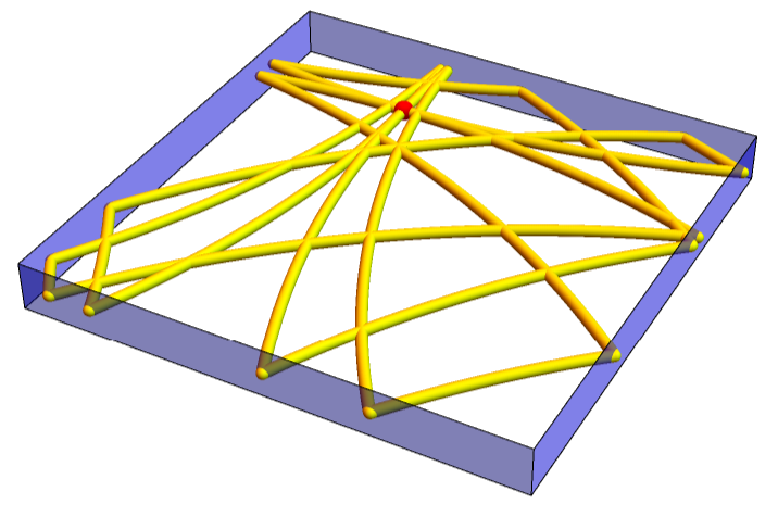
For the square it is simpler. And we can even use manipulate to
In[]:=
line[{X_,Y_}]:=If[(X-Y).(X-Y)>0.5,{Orange,Sphere[X,0.01]},{Yellow,Tube[{X,Y},0.01]}];mod[{x_,y_,z_}]:=Module[{},{X,Y}=Mod[{x,y},2];If[X<=1&&Y<=1,{a,b}=Mod[{X,Y},1]];If[X<=1&&Y>1,{a,b}={X,2-Y}];If[X>1&&Y<=1,{a,b}={2-X,Y}];If[X>1&&Y>1,{a,b}={2-X,2-Y}];{a,b,0}];h=0.05;P={0.3234234,0.823234,0};T0={Red,Sphere[P,0.02]};T1={Blue,Opacity[0.5],Polygon[{{0,0,-h},{1,0,-h},{1,0,h},{0,0,h},{0,0,-h}}]};T2={Blue,Opacity[0.5],Polygon[{{0,0,-h},{0,1,-h},{0,1,h},{0,0,h},{0,0,-h}}]};T3={Blue,Opacity[0.5],Polygon[{{0,1,-h},{1,1,-h},{1,1,h},{0,1,h},{0,1,-h}}]};T4={Blue,Opacity[0.5],Polygon[{{1,0,-h},{1,1,-h},{1,1,h},{1,0,h},{1,0,-h}}]};WW[R_,dt_]:=Module[{A,r},r[t_]:=mod[P+{R*Cos[t],R*Sin[t],0}];A=Table[line[{r[t],r[t+dt]}],{t,0,2Pi,dt}];Graphics3D[{T0,T1,T2,T3,T4,A},Boxed->False]];H[t_]:=WW[t,0.002];H[2.0]
Out[]=
References
References
[1] E. Kang and O. Knill, Density of Wave fronts https://arxiv.org/abs/2501.14611 , 2025
[2] Oliver Knill: Differential Geometry on Finite Sets, https://youtu.be/s0pvboRtiHs?si=vThAHYgspcefsbtB&t=383
[2] Oliver Knill: Differential Geometry on Finite Sets, https://youtu.be/s0pvboRtiHs?si=vThAHYgspcefsbtB&t=383
CITE THIS NOTEBOOK
CITE THIS NOTEBOOK
Density of wave fronts: flat tori proof extends to cube, square & Klein
by Emily Kang & Oliver Knill
Wolfram Community, STAFF PICKS, April 9, 2025
https://community.wolfram.com/groups/-/m/t/3442267
by Emily Kang & Oliver Knill
Wolfram Community, STAFF PICKS, April 9, 2025
https://community.wolfram.com/groups/-/m/t/3442267