Comparison of CO2 depletion for various flow patterns
Authors: Housam Binous and Ahmed Bellagi
Comparison of CO2 depletion for various flow patterns
Authors: Housam Binous and Ahmed Bellagi
Authors: Housam Binous and Ahmed Bellagi
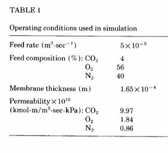
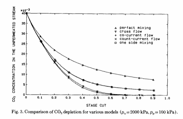
Various flow patterns for gas permeation of a multicomponent system are studied in Ref. 1. The feed is composed of CO2, O2, and N2, with an initial CO2 content of 4 mole % (see Table 1 of Ref. 1). The CO2 removal from closed or semi-closed life sustaining environments is considered. The objective is to achieve a lean stream content of CO2 of about 0.5 mole % in the breathing gas. Figure 3 of Ref. 1 depicts the CO2 concentration in the retentate stream versus stage cut for five flow patterns.Here, we successfully reproduce Fig. 3 of Ref. 1 using the methodology described in detail in Ref. 2.References:[1] K. Li, D.R. Acharya, R. Hughes, Mathematical modelling of multicomponent membrane permeators, Journal of Membrane Science, Volume 52, Issue 2, 1990, Pages 205-219, https://doi.org/10.1016/S0376-7388(00)80486-X .[2] H . Binous, U . Zahid and A . Bellagi, Modeling for Multi - component Gas Permeation with Orthogonal Collocation and Arc - Length Continuation, Chemistry Africa (2024) . https://doi.org/10.1007/s42250-024-01167-y
In[]:=
functions={xA[1]xA[1][s],yAyA[s],xB[1]xB[1][s],yByB[s],xA[2]xA[2][s],yA[2]yA[2][s],xB[2]xB[2][s],yB[2]yB[2][s],q[2]q[2][s],xA[3]xA[3][s],yA[3]yA[3][s],xB[3]xB[3][s],yB[3]yB[3][s],q[3]q[3][s],xA[4]xA[4][s],yA[4]yA[4][s],xB[4]xB[4][s],yB[4]yB[4][s],q[4]q[4][s],xA[5]xA[5][s],yA[5]yA[5][s],xB[5]xB[5][s],yB[5]yB[5][s],q[5]q[5][s],xA[6]xA[6][s],yA[6]yA[6][s],xB[6]xB[6][s],yB[6]yB[6][s],q[6]q[6][s],xA[7]xA[7][s],yA[7]yA[7][s],xB[7]xB[7][s],yB[7]yB[7][s],q[7]q[7][s],xA[8]xA[8][s],yA[8]yA[8][s],xB[8]xB[8][s],yB[8]yB[8][s],q[8]q[8][s],xA[9]xA[9][s],yA[9]yA[9][s],xB[9]xB[9][s],yB[9]yB[9][s],q[9]q[9][s],xA[10]xA[10][s],yA[10]yA[10][s],xB[10]xB[10][s],yB[10]yB[10][s],q[10]q[10][s],xA[11]xA[11][s],yA[11]yA[11][s],xB[11]xB[11][s],yB[11]yB[11][s],q[11]q[11][s],xA[12]xA[12][s],yA[12]yA[12][s],xB[12]xB[12][s],yB[12]yB[12][s],q[12]q[12][s],xA[13]xA[13][s],yA[13]yA[13][s],xB[13]xB[13][s],yB[13]yB[13][s],q[13]q[13][s],xA[14]xA[14][s],yA[14]yA[14][s],xB[14]xB[14][s],yB[14]yB[14][s],q[14]q[14][s],xA[15]xA[15][s],yA[15]yA[15][s],xB[15]xB[15][s],yB[15]yB[15][s],q[15]q[15][s],xA[16]xA[16][s],yA[16]yA[16][s],xB[16]xB[16][s],yB[16]yB[16][s],q[16]q[16][s],xA[17]xA[17][s],yA[17]yA[17][s],xB[17]xB[17][s],yB[17]yB[17][s],q[17]q[17][s],xA[18]xA[18][s],yA[18]yA[18][s],xB[18]xB[18][s],yB[18]yB[18][s],q[18]q[18][s],xA[19]xA[19][s],yA[19]yA[19][s],xB[19]xB[19][s],yB[19]yB[19][s],q[19]q[19][s],xA[20]xA[20][s],yA[20]yA[20][s],xB[20]xB[20][s],yB[20]yB[20][s],q[20]q[20][s],xA[21]xA[21][s],yA[21]yA[21][s],xB[21]xB[21][s],yB[21]yB[21][s],q[21]q[21][s],q[1]q[1][s],thetatheta[s],stst[s]};
ONE SIDE MIXING
ONE SIDE MIXING
In[]:=
x
fA
x
fB
x
fC
q
P
q
f
q
f
p
l
p
h
Np+1
∑
j=1
Np+1
∑
j=1
Np+1
∑
j=1
Np+1
∑
j=1
p
l
p
h
p
l
p
h
p
l
p
h
p
l
p
h
p
l
p
h
p
l
p
h
p
l
p
h
p
l
p
h
p
l
p
h
p
l
p
h
p
l
p
h
x
fA
x
fB
x
fA
x
fB
Out[]=
{xA[1]0.0210518,xB[1]0.547541,xA[2]0.0211304,xB[2]0.547655,xA[3]0.0213665,xB[3]0.547992,xA[4]0.0217611,xB[4]0.548535,xA[5]0.0223155,xB[5]0.54926,xA[6]0.0230302,xB[6]0.550135,xA[7]0.0239042,xB[7]0.551122,xA[8]0.0249335,xB[8]0.552179,xA[9]0.0261096,xB[9]0.553264,xA[10]0.0274184,xB[10]0.554337,xA[11]0.0288388,xB[11]0.555361,xA[12]0.0303417,xB[12]0.556308,xA[13]0.0318902,xB[13]0.557156,xA[14]0.0334395,xB[14]0.557889,xA[15]0.0349391,xB[15]0.558503,xA[16]0.0363344,xB[16]0.558998,xA[17]0.0375705,xB[17]0.559381,xA[18]0.0385952,xB[18]0.559663,xA[19]0.0393631,xB[19]0.559854,xA[20]0.0398389,xB[20]0.559964,q[2]0.847232,q[3]0.849897,q[4]0.854277,q[5]0.860276,q[6]0.867767,q[7]0.876586,q[8]0.88654,q[9]0.897406,q[10]0.908938,q[11]0.920866,q[12]0.932905,q[13]0.944762,q[14]0.956135,q[15]0.96673,q[16]0.97626,q[17]0.984463,q[18]0.991106,q[19]0.995997,q[20]0.998992,yA0.144362,yB0.628619,theta0.153663}
In[]:=
xA[Np+1]=.;xB[Np+1]=.;q[Np+1]=.;q[1]=.;init=Join[Flatten[Table[{xA[i][0](xA[i]/.sol),xB[i][0](xB[i]/.sol)},{i,1,Np}],1],Flatten[Table[q[i][0](q[i]/.sol),{i,2,Np}],1],{xA[Np+1][0]==,xB[Np+1][0]==,q[Np+1][0]==1,q[1][0]==(1-theta/.sol),theta[0](theta/.sol),st[0]1,yA[0](yA/.sol),yB[0](yB/.sol)}];initdev=Join[Flatten[Table[{xA[i]'[0]0.001,xB[i]'[0]0.001},{i,1,Np+1}],1],Flatten[Table[{q[i]'[0]0.1},{i,1,Np+1}],1],{theta'[0]100,st'[0]1,yA'[0]-0.1,yB'[0]-0.1}];aux=Sum[xA[i]'[s]^2+xB[i]'[s]^2,{i,1,Np+1}]+Sum[q[i]'[s]^2,{i,1,Np+1}]+yA'[s]^2+yB'[s]^2+theta'[s]^2+st'[s]^21;unknown1=Join[Flatten[Table[{xA[i],xB[i]},{i,1,Np+1}],1],Flatten[Table[q[i],{i,1,Np+1}],1],{theta,st,yA,yB}];SYS=Join[sys/.functions,{aux,xA[Np+1][s]==,xB[Np+1][s]==,q[Np+1][s]==1,q[1][s]==(1-theta[s])},init,initdev];SOL=Quiet@NDSolve[SYS,unknown1,{s,-100,100},AccuracyGoal7];p1=ParametricPlot[Evaluate[{theta[s],10^3xA[1][s]}/.SOL[[1]]],{s,-100,10},PlotRange{{0.00,1.0},{0,40}},FrameTrue,GridLinesAutomatic,AspectRatio1,PlotStyle{Red,Dashed,Thick},FrameTrue,FrameLabel{Style["stage cut",16],Style["CO2 in reject",16]}];
x
fA
x
fB
x
fA
x
fB
PERFECT MIXING
PERFECT MIXING
CO-CURRENT
CO-CURRENT
CROSS-FLOW
CROSS-FLOW
COUNTER-CURRENT
COUNTER-CURRENT
Comparison with Figure 3 of Li et al .
Comparison with Figure 3 of Li et al .