Black holes (BHs) have the strongest gravitational force in the observable universe. This study investigates the effects of Schwarzschild and Kerr black holes (BH) on matter by considering general relativity and the curvature of spacetime. It explores a way to quantify spaghettification and models the effects from both types of black holes. Additionally, it also models different in-falls (polar and equatorial)/trajectories for structures approaching black holes and compares the spaghettification of both of them. It uses geodesic equations, Christoffel symbols and a metric tensor to create these models for both types of black holes.
Introduction
Introduction
A black hole is what is formed when a massive star collapses at the end of its lifetime or when a vast amount of matter is crushed into an extremely small, dense area. Its immense gravitational force pulls in all things that come near it and it becomes impossible for them to escape, after a point (the event horizon) even light cannot escape.
The singularity of a black hole is a theoretical point (usually) located at its center. As matter moves closer to the singularity, the gravitational force grows stronger due to the curvature of space-time. So if there was an object approaching a black hole, the end that is closer to the black hole would experience more gravitational force than the other far end, this would cause the object to stretch towards the BH, an effect known as spaghettification. In this project, I will delve into the effects of spaghettification from non-spinning BH (Schwarzschild) and spinning BH (Kerr BH), explore a method to quantify spaghettification, and lastly, polar and equatorial in-fall.
In order to accurately model black holes, Newton’s equations cannot be used because the gravitational field is nothing close to uniform. Therefore, this project will use Einstein’s theory of general relativity that explains gravitational field through space-time.
In order to accurately model black holes, Newton’s equations cannot be used because the gravitational field is nothing close to uniform. Therefore, this project will use Einstein’s theory of general relativity that explains gravitational field through space-time.
What is Spaghettification?
What is Spaghettification?
As you approach the center of the black hole, the volume of matter keeps reducing and the matter becomes more and more dense. Eventually in the center of the BH the volume of matter is zero so its density is infinite, this point is called the singularity of the BH.
As matter moves closer to the singularity, the gravitational force grows stronger due to the curvature of space-time; so if there was an object approaching the BH, the end that is closer to the black hole would experience more gravitational pull compared to the far end, this would cause the object to stretch towards the BH. This net force is known as the tidal force.
The tidal force increases significantly as the matter moves closer to the singularity. This vertical stretching (and horizontal compression) effect is known as spaghettification.
In[]:=
G=Quantity["GravitationalConstant"];
In[]:=
M=10^30;
In[]:=
m=10^6;
In[]:=
h=100;
This graph models the tidal force, (y-axis) against the R, the distance between the singularity and the object (x-axis).
Graphing tidal force against R.
In[]:=
Plot,{R,0,20}
2G*M*m*h
3
R
Out[]=
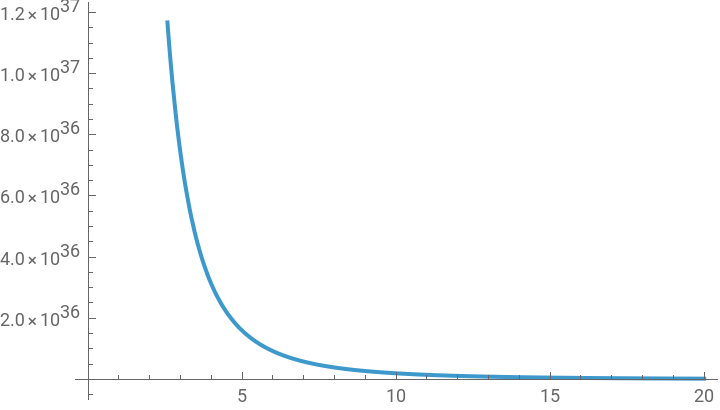
The effect of tidal force is like the simplified (Newtonian) version of what happens to objects when they approach a black hole. The difference in experience of gravitational force at two different points is what causes spaghettification.
The Mathematics Of General Relativity
The Mathematics Of General Relativity
The formula given for tidal force above is an explanation from Newton’s laws; it cannot be used to calculate for particles around a BH because in space-time the gravitational force is different at all points, even points on the same side. Therefore, I used geodesics.
Geodesics are the shortest paths between points along a spherical surface (in this case, space-time).
To model the effects on particles due to a BH gravity, I cannot use Newton’s equations and model gravity as a force, instead I have to model gravitational field in space-time. Therefore, for this project I used a space-time metric, in this case a Schwarzschild metric and a Kerr metric.
Schwarzschild Metric
Schwarzschild Metric
For a static, spherically symmetric, non-rotating mass, that metric is the Schwarzschild metric.
Clearing variables.
In[]:=
ClearAll[t,r,θ,ϕ,coords,schwarzschildMetric,M];coords={t,r,θ,ϕ};
Importing the resource function of the metric for Schwarzschild.
In[]:=
schwarzschildMetric=[{"Schwarzschild",M},coords]/.{M->1};MatrixForm[schwarzschildMetric["MatrixRepresentation"]/.{M->1}]
Out[]//MatrixForm=
-1+ 2 r | 0 | 0 | 0 |
0 | 1 1- 2 r | 0 | 0 |
0 | 0 | 2 r | 0 |
0 | 0 | 0 | 2 r 2 Sin[θ] |
Showing the tensor rank, which indicates how many indices are needed to specify a symbol.
In[]:=
TensorRank[Γs]
Out[]=
3
Showing the tensor dimensions of the matrix.
In[]:=
TensorDimensions[Γs]
Out[]=
{4,4,4}
From the Schwarzschild metric I compute the Christoffel symbols. These coefficients tell me how vectors are parallel transported and how coordinates curve. Parallel transporting a vector means moving it along a curve without changing its length or direction relative to the curved space. They are the ingredients needed to write the geodesic equations for free fall.
In[]:=
christoffel=[schwarzschildMetric];Γs=christoffel["ReducedTensorRepresentation"];
Displaying the matrix.
In[]:=
MatrixForm[Γs]
Out[]//MatrixForm=
|
|
|
| ||||||||||||||||
|
|
|
| ||||||||||||||||
|
|
|
| ||||||||||||||||
|
|
|
|
This tells me how vectors change from one point to another in spacetime and how to write the geodesic equations.
In[]:=
ThetypicalindexstructureforChristoffelsymbolsis:.Theouterblockintheindexcorrespondstoμandthebottomtworepresentthematrixinνandρ.
μ
Γ
νρ
◼
μ = t: time equation
◼
μ = r: radial equation
◼
μ = θ: polar-angle equation
◼
μ = ϕ: azimuthal-angle equation
These all become functions of time from a observational point very far away from the BH where it cannot feel its gravitational effects.
Kerr Metric
Kerr Metric
For a rotating black hole, that metric is the Kerr metric.
In[]:=
kerrMetric=[{"Kerr",M,J},coords];MatrixForm[kerrMetric["MatrixRepresentation"]/.{M->1}]
Out[]//MatrixForm=
-1+ 2r 2 r 2 J 2 Cos[θ] | 0 | 0 | - 2Jr 2 Sin[θ] 2 r 2 J 2 Cos[θ] |
0 | 2 r 2 J 2 Cos[θ] 2 J 2 r | 0 | 0 |
0 | 0 | 2 r 2 J 2 Cos[θ] | 0 |
- 2Jr 2 Sin[θ] 2 r 2 J 2 Cos[θ] | 0 | 0 | 2 Sin[θ] 2 J 2 r 2 2 J 2 Sin[θ] 2 r 2 J 2 Cos[θ] |
Geodesic Equations
Geodesic Equations
So, I replaced Newtons equations of motion with this geodesic that free-falling particles follow around a Schwarzschild BH.+0.
2
d
μ
x
d
2
τ
μ
Γ
νρ
d
ν
x
dτ
d
ρ
x
dτ
Setting up geodesic equations.
In[]:=
geodesicEquations=Table[coords[[mu]]''[τ]+Sum[(Γs[[mu,nu,rho]]/.Thread[coords->Through[coords[τ]]])*coords[[nu]]'[τ]*coords[[rho]]'[τ],{nu,4},{rho,4}]==0,{mu,4}];
In[]:=
geodesicEquations
Out[]=
+[τ]0,[τ]++(2-r[τ])[τ]-(-2+r[τ])[τ]+[τ]0,-Cos[θ[τ]]Sin[θ[τ]][τ]+[τ]0,+2Cot[θ[τ]][τ][τ]+[τ]0
2[τ][τ]
′
r
′
t
(-2+r[τ])r[τ]
′′
t
2
′
r
2r[τ]-
2
r[τ]
(-2+r[τ])[τ]
2
′
t
3
r[τ]
2
′
θ
2
Sin[θ[τ]]
2
′
ϕ
′′
r
2[τ][τ]
′
r
′
θ
r[τ]
2
′
ϕ
′′
θ
2[τ][τ]
′
r
′
ϕ
r[τ]
′
θ
′
ϕ
′′
ϕ
I set to make this model two dimensional and only in the equatorial plane. This works because Schwarzschild spacetime is spherically symmetric so I can rotate a geodesic into a plane.
θπ/2
Reducing the geodesic equations.
reducedEquations=DeleteCases[ReplaceAll[geodesicEquations,{θ[τ]->Pi/2,θ'[τ]->0,θ''[τ]->0}],True];
Solving the equations.
Now I can plot the path of the orbit around a Schwarzschild BH which is the geodesic:
Plotting a Schwarzschild geodesic.
This image may resemble a central-force trajectory, but it contains more interesting physics than a Newtonian orbit:
◼
the time coordinate t[τ] evolves dynamically
◼
the motion is derived from the spacetime metric, not from a force law
◼
relativistic curvature corrections are built directly into the radial and angular equations
◼
the path is parameterized by proper time, the time experienced by the falling particle
Spaghettification Demo in 2D
Spaghettification Demo in 2D
Spaghettification can be visualized by making a shape/blob using many points which will all have different geodesics to each other and different initial positions (some closer the the BH than others) which will cause them to separate from each other unequally.
Initial Blob Shapes
Initial Blob Shapes
Defining the function “createInitialBlob”.
These different 2D shapes made up of points is what I will demo spaghettification on. If you ever wondered what would happen to you if you entered a black hole... you can imagine yourself as the stick figure shape.
Solve Timelike Geodesic
The function ‘solveTimelikeGeodesic2D’ takes geodesic equations, the metric, max. time, initial positions and the spin J of the BH.
It outputs the solution which is an interpolating function for {t, r, ϕ} for a given initial point.
It outputs the solution which is an interpolating function for {t, r, ϕ} for a given initial point.
Creating the function.
The initial condition for the first time derivative of time was computed from the metric.
Square
Square
Schwarzschild
Schwarzschild
Using ‘With’ to combine all the functions and create the final graphic.
For the Kerr BH, I explored the visualization for a low spin (J=0.4) and a high spin (J=0.999).
The value of J has to be kept less than M because when J>M the event horizon of the BH disappears and the BH turns into something called a naked singularity with infinite density. Although this is mathematically possible, it is believed not to exist in reality.
The value of J has to be kept less than M because when J>M the event horizon of the BH disappears and the BH turns into something called a naked singularity with infinite density. Although this is mathematically possible, it is believed not to exist in reality.
Kerr: J=0.4
Kerr: J=0.4
Kerr: J=0.999
Kerr: J=0.999
By comparing the visuals for both the spins, I can see that J=0.999 wraps around the BH all the way in the direction of the spin (indicated by the red arrow). Whereas with J=0.4 it only wraps a limited amount. This is due to an effect known as ‘frame-dragging’. This is a phenomenon seen in spinning BH where the mass pulls spacetime with it as it rotates.
By comparing the visuals for both the spins, I can see that J=0.999 wraps around the BH all the way in the direction of the spin (indicated by the red arrow). Whereas with J=0.4 it only wraps a limited amount. This is due to an effect known as ‘frame-dragging’. This is a phenomenon seen in spinning BH where the mass pulls spacetime with it as it rotates.
Circle
Circle
Schwarzschild
Schwarzschild
Kerr: J=0.4
Kerr: J=0.4
Kerr: J=0.999
Kerr: J=0.999
Line
Line
Schwarzschild
Schwarzschild
Observe how the center part of the line is pulled in more than the ends, showing obvious spaghettification.
Kerr: J=0.4
Kerr: J=0.4
Kerr: J=0.999
Kerr: J=0.999
Stick Man
Stick Man
Lastly, this is what could happen to you if you venture too deep into space...
Schwarzschild
Schwarzschild
Kerr: J=0.4
Kerr: J=0.4
Kerr: J=0.999
Kerr: J=0.999
Quantification of Spaghettification in 2D
Quantification of Spaghettification in 2D
It was very satisfying to see a working model of spaghettification and see how the blob stretches... However, I wanted to find a way to measure it and quantify spaghettification so that I can compare different conditions and initial start positions (will be explored in 3D later on).
Creating the function “quantifySpaghettification2D”.
The way that I quantified it was for an multiple instants in time, I calculated the average Euclidean distance between all the points in the shape/blob at that instant. Then displayed it as a graph. This graph is comparing the “Circle” shape for the Schwarzschild BH with the Kerr BH (with J=0.999).
There is a negligible difference between these two.
Visualizing Spaghettification in 3D Through Polar and Equatorial Infalls
Visualizing Spaghettification in 3D Through Polar and Equatorial Infalls
When I visualize spaghettification in 3D, it matters where I drop the particles from because the effect would differ if dropped it from the poles or from somewhere in the equatorial plane because I am considering that the spin is in the equatorial plane. I explored the effects of both of these. However, this theory would only hold true for Kerr BHs because technically a Schwarzschild BH does not have poles as it is a symmetrical sphere with zero spin.
Define Functions For 3D
Define Functions For 3D
The function ‘solveTimelikeGeodesic3D’ takes equations, metric type, max. time and t, r, θ, ϕ at 0 as inputs and it solves the geodesic equations but this time including a third dimension. In this demo, I will consider initial angular velocity equal to zero.
Setting up the function ‘solveTimelikeGeodesics3D’.
Creating the function ‘spaghettify3D’ which solves the geodesic equations.
In order to plot the graphics, Cartesian form is needed.
Making the function ‘kerrToCartesian’.
Defining the function ‘visualizeSpaghettification3D’.
Define Blobs
Define Blobs
Equatorial:
Equatorial:
This is a blob on the x-axis.
Polar:
Polar:
This is a spherical blob on the z-axis.
Quantify Spaghettification 3D
Quantify Spaghettification 3D
To quantify spaghettification for 3D I used the same method as I did for 2D of finding the average distance between the coordinates of all the points in the blob/shape.
Making the function ‘quantifySpaghettification3D’.
Schwarzschild
Schwarzschild
Equatorial
Equatorial
Over here the particles all go straight to the center of gravity of the BH as they get stretched out.
Polar
Polar
Making a plot to demonstrate spaghettification in equatorial and polar planes.
As predicted earlier, you can tell that the spaghettification effect is the same when the particle is dropped from the pole and when it is dropped in the equatorial plane for the Schwarzschild BH.
However, this should not be the case for a Kerr BH because the spin axis of the BH is the equatorial plane.
However, this should not be the case for a Kerr BH because the spin axis of the BH is the equatorial plane.
Kerr
Kerr
Equatorial
Equatorial
Using ‘With’ to output the graphic of spaghettification on the equatorial axis for a Kerr BH.
The points warp around the BH in the direction of it’s spin, which is once again the effect of frame-dragging.
Modelling spaghettification for a Kerr BH for objects dropping from one of the poles of the BH.
Polar
Polar
So, when points fall from above a pole of the Kerr BH then the particles do not circle the BH, they just go straight to the center of mass of the BH. This effect is similar to the effect seen for Schwarzschild BH. This is because there is no spin so no frame-dragging in the polar plane and there is no initial angular velocity.
To compare the spaghettification of when particles fall from the equatorial plane versus when they fall from the polar plane in Kerr BH, I plotted a graph with spaghettification on the y-axis and time on the x-axis.
To compare the spaghettification of when particles fall from the equatorial plane versus when they fall from the polar plane in Kerr BH, I plotted a graph with spaghettification on the y-axis and time on the x-axis.
Plotting the two spaghettifications for Kerr BHs.
Here it can be seen that at first spaghettification is more in the polar plane but at around time=14 the spaghettification that takes place in the equatorial plane overtakes the polar plane. This is due to the frame-dragging effect (only experienced in the equatorial plane) getting stronger as the points move closer to the BH.
Spaghettifying a Bunny
Spaghettifying a Bunny
Now that you (stick man) have seen what happens when you enter a BH, what about your pet bunny?
Importing the Stanford Bunny.
Taking random points from the structure.
Making a cloud of of the structure and spaghettifying it using ‘spaghettify3D’.
The bunny wrapped all the way around the BH and is now “spaghettified”.
Conclusion & Future Directions
Conclusion & Future Directions
The major conclusion from this project is the difference in spaghettification of particles/blobs when they fall into Kerr black holes at the polar plane and the equatorial plane due to the effect of frame-dragging.
I have also visually verified the effect of varying the spin parameter J by observing frame-dragging.
In this project, thanks to Wolfram Language, I used Resource Functions for the metric tensor and Christoffel symbols which was the backbone for the code of this project. This saved me a lot of time and allowed me to allocate my time to focus on using the functions to model things instead of coding them.
To take this project further, I hope to model mega-structures and analyze the forces that are experienced within the structure. For example, how the tensile strength of a structure compares to the tidal forces on it due to a BH.
Furthermore, I would like to explore different ways to quantify spaghettification by other means such as finding the area and volume of the structure and plot them against time.
Lastly, I would like to model spaghettification and orbits using values of angular velocity (greater than zero). This could be incorporated into one of the existing functions from this project.
Acknowledgements
Acknowledgements
Firstly, a huge thank you to my mentor and advocate, Joseph Brennan, for carrying me through this project through his immense help and guidance throughout this project, always answering my questions with patience and for our shared excitement about this project. I would also like to thank the program directors, Rory, Eryn and Megan for their continuous support. I am forever grateful to Stephen Wolfram for this opportunity, giving me and helping me figure out this project and making complex concepts understandable when he explains them.
References
References
CITE THIS NOTEBOOK
CITE THIS NOTEBOOK
Exploring spaghettification around black holes
by Aanya Sinha
Wolfram Community, STAFF PICKS, July 9, 2026
https://community.wolfram.com/groups/-/m/t/3753652
by Aanya Sinha
Wolfram Community, STAFF PICKS, July 9, 2026
https://community.wolfram.com/groups/-/m/t/3753652