ORIGINAL ARTICLE: Gerhard C. Hegerfeldt, Time-Optimal Transport of a Harmonic Oscillator: Analytic Solution, Phys. Scr. 98 (2023) 095101, DOI: https://doi.org/10.1088/1402-4896/ace999
Introduction
Introduction
Motivated by the experimental transport of a trap with a quantum mechanical system modeled as a harmonic oscillator (h.o.) the corresponding classical problem is investigated. We consider a classical one-dimensional harmonic oscillator (h.o.) without friction in the center of a long wagon, where a small mass is attached to a spring on the wagon. When the wagon is accelerated the h.o. will start to perform oscillations. In this case the frequency Ω of the h.o. depends on the spring constant and on .
m
m
The problem:
The problem:
1
.Initially the wagon is at rest and the h.o. is in its equilibrium position, also at rest.
2
.Then the wagon undergoes an acceleration , where can vary between , until it has traveled a prescribed distance .
a(t)
a(t)
±
a
max
d
3
.Upon arrival at the end point the wagon should be at rest, and the h.o. should again be in its equilibrium position and at rest.
Is this achievable? And if so what is the shortest time possible? Can this time be further lowered by allowing the h.o. frequency Ω to be time dependent, i.e. ? These questions are answered in the affirmative in [1].
Ω(t)
Fixed oscillator frequency
Fixed oscillator frequency
x
h
x
w
̈
x
h
2
Ω
x
h
̈
x
w
Pontryagin Maximum Principle (PMP) [2] yields: is piecewise constant, = . Then the solution (t) is obtained from (t)+i (t)exp[-iΩ(t-)]·()+i ()±∓
a(t)
a(t)
±
a
max
x
h
x
h
-1
Ω
x
h
t
0
x
h
t
0
-1
Ω
x
h
t
0
a
max
2
Ω
a
max
2
Ω
Optimal procedure (“protocol”) for constant Ω [1] :
1
.For given determine the unique optimal time by the equation .
d
t
f
d1-
1
4
a
max
2
t
f
8
2
(Ω )
t
f
2
(arccos((Ω /4)))
2
cos
t
f
2
.With wagon and oscillator at rest at , accelerate with until time - where , , is given by arccos((Ω /4)).
t=0
a
max
1
2
t
f
t
1
t
1
0≤Ω≤π/2
t
1
t
1
1
Ω
2
cos
t
f
3
.Decelerate with until time .
-
a
max
1
2
t
f
4
.Accelerate with until time +.
a
max
1
2
t
f
t
1
5
.Finally decelerate with until time .
-
a
max
t
f
t
f
T
abs
d/
a
max
In[]:=
<<MaTeX`
In[]:=
g=InverseFunction-8&;
1
4
2
#
2
ArcCos
2
Cos
#
4
In[]:=
Plot[{2*Sqrt[4Pi^2*s],g[4Pi^2*s]},{s,0,4},PlotLegendsPlaced[{MaTeX["T_{\\rm abs}"],MaTeX["t_{\\rm f}(d)"]},Scaled[{0.8,0.5}]],Axes->True,PlotStyle->{Dashed,Solid},AxesLabel{MaTeX["d/d_\\Omega",Magnification1.1],MaTeX[" {\\rm time}/\\Omega^{-1}",Magnification1.1]},AspectRatio1]
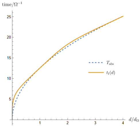
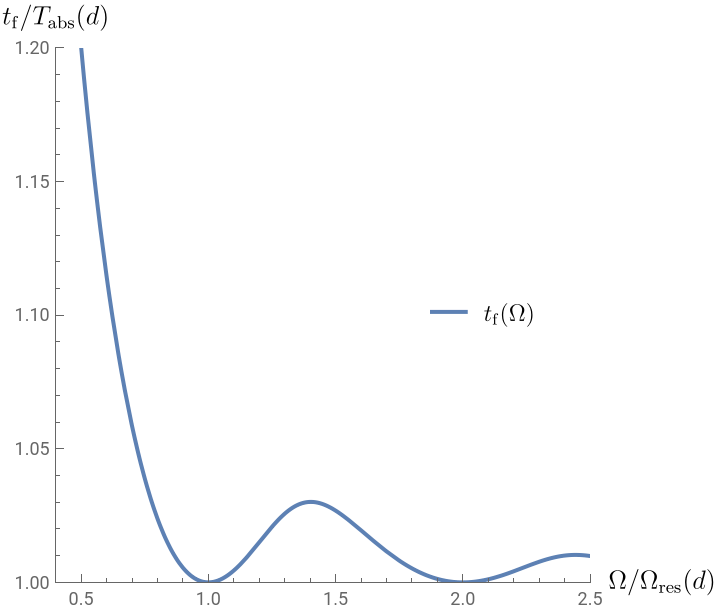
With (d)4π/ one obtains as a function of Ω:
Ω
res
T
abs
t
f
In[]:=
Plot[1/4/Pi/s*g[4Pi^2*s^2],{s,.05,2.5},PlotLegendsPlaced[{MaTeX["t_{\\rm f}(\\Omega)"]},Scaled[{0.8,0.5}]],AxesLabel{MaTeX["\\Omega /\\Omega_{\\rm res}(d) ",Magnification1.1],MaTeX["t_{\\rm f}/T_{\\rm abs}(d)",Magnification1.1]},PlotRange{{.4,2.5},{1,1.2}},AspectRatio1]
Out[]=
Time-dependent oscillator frequency
Time-dependent oscillator frequency
0≤≤Ω(t)≤<∞
Ω
-
Ω
+
|a(t)|≤
a
max
Scaled variables: a fixed length unit, , ω(t)Ω(t)(τ)(t), (τ)(τ)(τ)(t), (τ)(τ)so that can vary between -1 and 1. Then≡-(τ)-u(τ)u(τ) .We choose =d. Then =2 and =2π.
d
0
2
Ω
0
a
max
d
0
Ω
0
τt, u(τ)a(t)/
Ω
0
a
max
ξ
1
x
h
d
0
ξ
2
d
dτ
ξ
1
ξ
3
x
w
d
0
ξ
4
d
dτ
ξ
3
u(τ)
̈
ξ
1
2
d
d
2
τ
ξ
1
2
ω
ξ
1
̈
ξ
3
d
0
τ
abs
ω
res
If lies in the interval for some then choosing will give the minimal time (d). Otherwise, PMP yields (with possible exceptions):
is piecewise constant, ,
is piecewise constant, .
n(d)
Ω
res
[,]
Ω
-
Ω
+
n
n(d)
Ω
res
T
abs
u(t)
u(t)±1
ω(t)
ω(t)
ω
±
There are switches in at /2 and /2± where both and are yet to be determined. The distance traveled in time is -2 and if is to be optimal it must satisfy (1) where =(,).
u
τ
f
τ
f
τ
1
τ
f
τ
1
τ
f
1
4
2
τ
f
2
τ
1
τ
f
d1-2
d
0
1
4
2
τ
f
2
τ
1
τ
f
τ
f
ω
-
ω
+
Case 0<ω-<ω+<ωres2π
Case
0<<<2π
ω
-
ω
+
ω
res
(i) If ≤π only enters and there is no switch in . This is the case of constant from above and the corresponding (,) is depicted in the next plot.
ω
+
ω
+
2
ω
+
ω
ω
t
f
Ω
+
Ω
-
In[]:=
Pab=ContourPlot3D[{(2*tauf)^2/4-2*1/(2*Pi*ompl)^2*ArcCos[Cos[2*Pi*ompl*2*tauf/4]^2]^2==1},{ompl,0,1},{ommi,0,1},{tauf,1,1.52},RegionFunctionFunction[{ompl,ommi,tauf},0<ommi<ompl<1&&ompl<=Sqrt[2]/4],RegionBoundaryStyleNone,ContourStyle{Directive[Green,Opacity[0.3]]},AxesLabel{MaTeX["\\Omega_+/\\Omega_{\\rm res}(d)",Magnification.9],MaTeX["\\Omega_-/\\Omega_{\\rm res}(d)",Magnification.9],MaTeX["t_{\\rm f}/T_{\\rm abs}(d)",Magnification.9]}]
Out[]=

(ii) If >π one starts with , continues with two complete periods, and finally switches to . /2 satisfies . Then has to satisfy .One now solves this equation together with Eq. (1) for under the condition that /2 lies in the last interval.
ω
+
2
ω
-
ω
+
ω
-
τ
f
π/≤/2≤π/+π/
ω
+
τ
f
ω
+
ω
-
τ
1
cos[]1+cos2+-π
ω
+
τ
1
2
ω
+
2
2
ω
-
ω
-
τ
f
ω
+
ω
-
ω
+
τ
f
τ
f
ω
-
These plots can be combined together with the upper, lower and diagonal boundary:
These plots can be combined together with the lower and diagonal boundary:
References
References
[1] G.C. Hegerfeldt, Phys. Scr. 98 (2023) 095101
[2] L.M. Hocking, Optimal Control: An Introduction to the Theory With Applications (Oxford: Clarendon Press 1991)
CITE THIS NOTEBOOK
CITE THIS NOTEBOOK
Optimal Transport of a Classical Harmonic Oscillator
by Gerhard C. Hegerfeldt
Wolfram Community, STAFF PICKS, October 13, 2023
https://community.wolfram.com/groups/-/m/t/3035725
by Gerhard C. Hegerfeldt
Wolfram Community, STAFF PICKS, October 13, 2023
https://community.wolfram.com/groups/-/m/t/3035725