CITE THIS NOTEBOOK: Wolfram R&D LIVE: xAct—efficient tensor computer Algebra by Jose Martin-Garcia. Wolfram Community DEC 1 2022.
CITE THIS NOTEBOOK: Wolfram R&D LIVE: xAct—efficient tensor computer Algebra by Jose Martin-Garcia. Wolfram Community DEC 1 2022.
Plan of the talk
Plan of the talk
◼
1. Introduction to xAct
◼
2. Abstract computations with xTensor
◼
3. Component computations with xCoba
◼
4. Perturbation examples with xPert and xTras
◼
5. Frequent questions and future plans
1. Introduction to xAct
1.1. Main
1.1. Main
◼
Project developed since 2002, all in Wolfram Language, with a bit of C code.
◼
xAct is a hierarchical collection of packages, currently 23. Several more soon.
◼
Performs both abstract computations and component computations, possibly mixed.
◼
◼
950+ different authors. Highest numbers of publications using xAct packages:
1.2. Resources
1.2. Resources
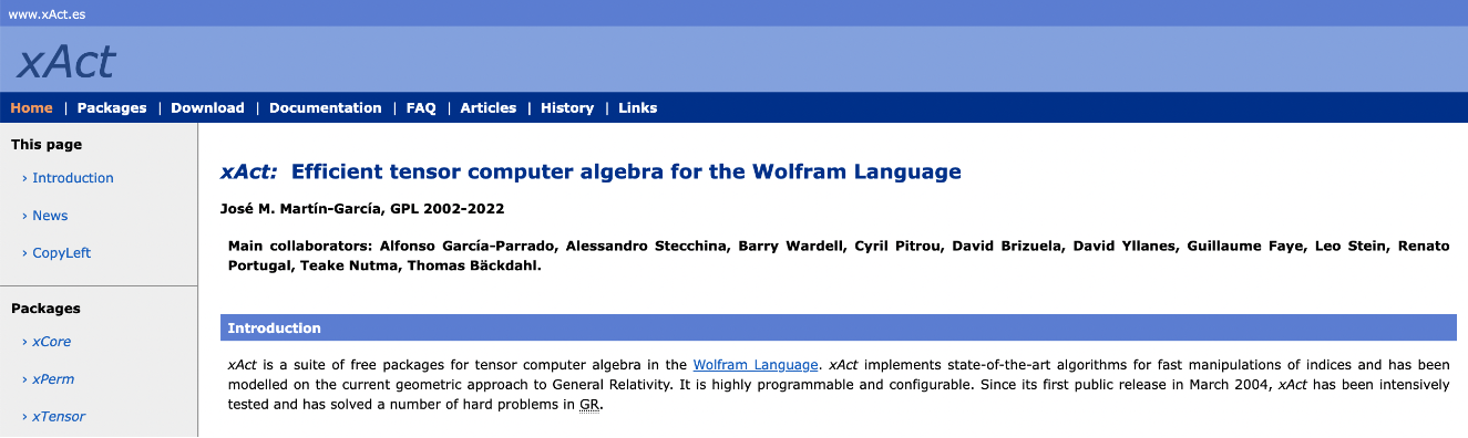
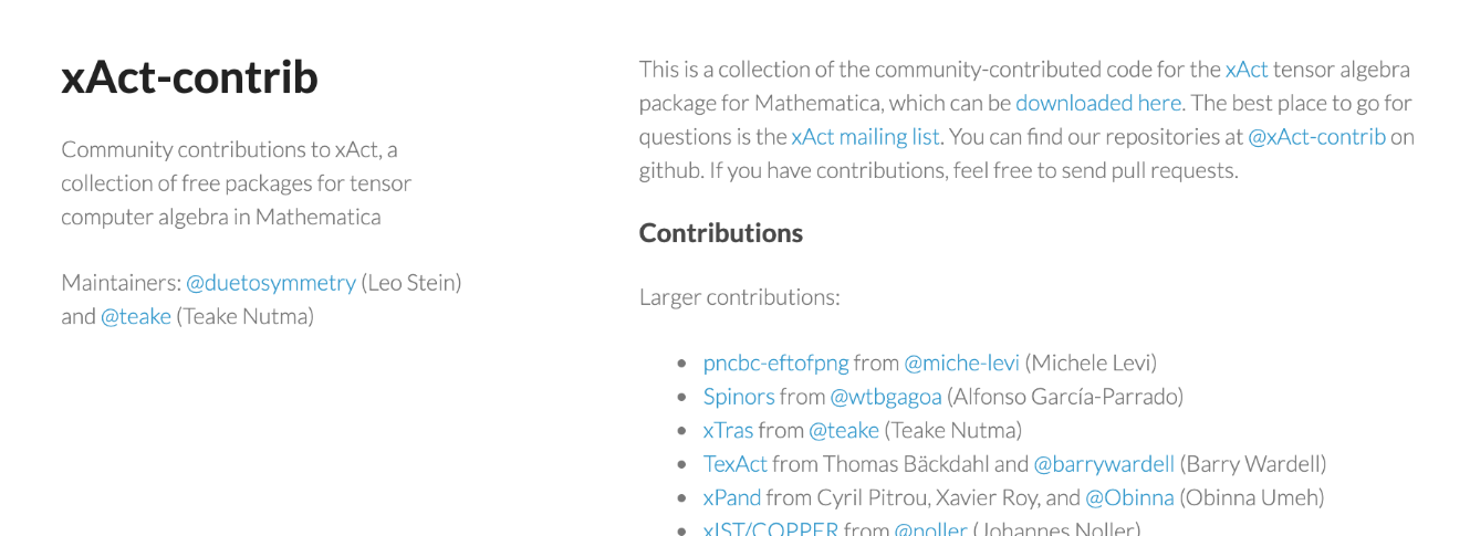
◼
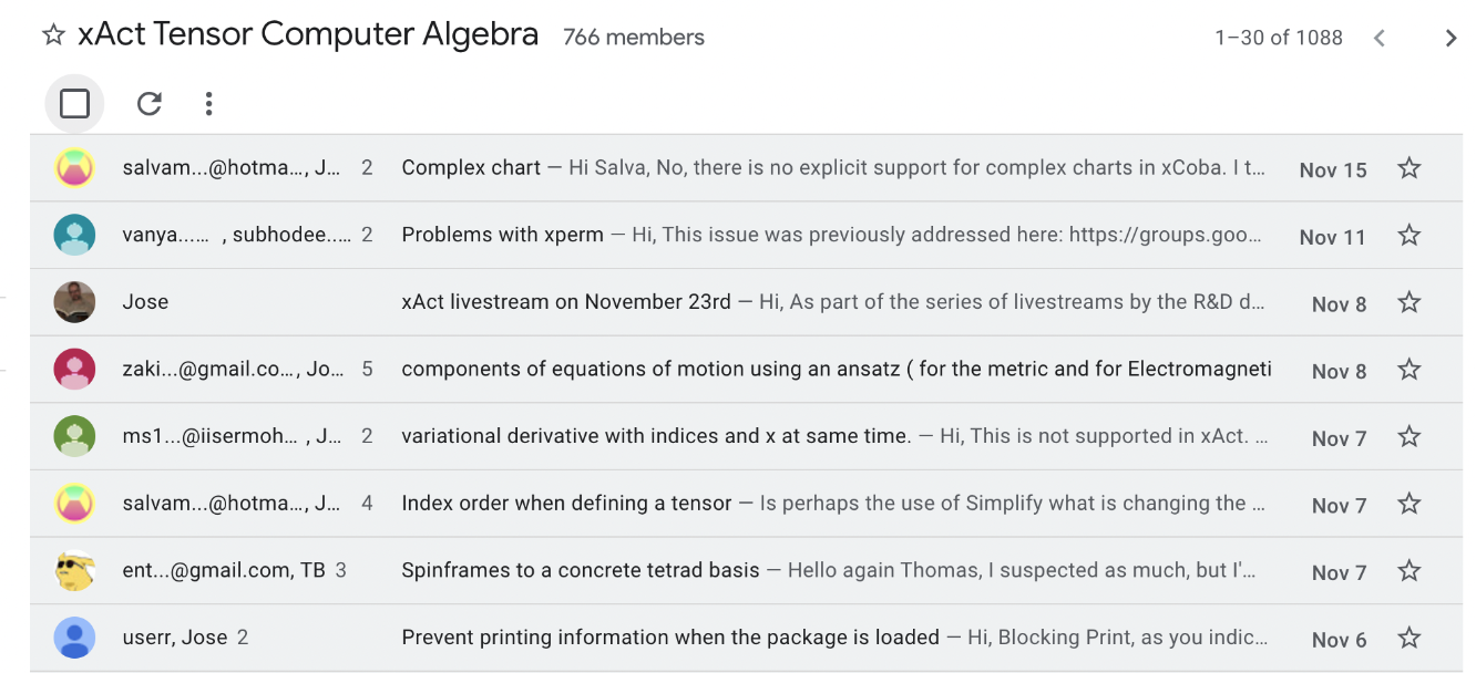
The xAct forum: [https://groups.google.com/g/xact]
◼
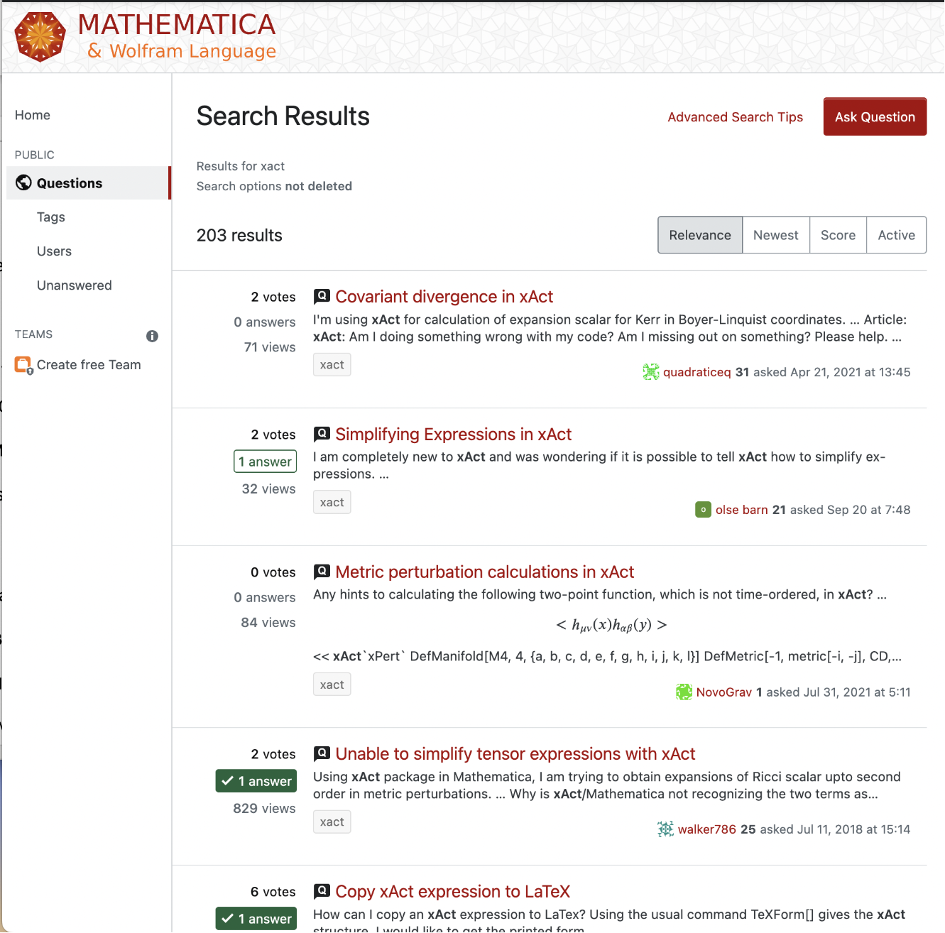
1.3. The structure of xAct
1.3. The structure of xAct
◼
xAct is a collection of packages, currently 23, organized hierarchically.
◼
When you load a package, all dependencies are loaded too.
◼
There are about 1500 xAct symbols in total, 450 of them just in xTensor.
Packages
Packages
Core packages
Core packages
Application packages
Application packages
Input/Output packages
Input/Output packages
Exceptional packages
Exceptional packages
Dependency graph
Dependency graph
• Loops are not allowed. All dependencies must point downwards:
1.4. Example session. Abstract versus component computations
1.4. Example session. Abstract versus component computations
Abstract computations
Abstract computations
◼
Deal with tensor expressions and identities that are independent of choices of frames and/or coordinates.
• Load xTensor:
• Define a manifold, two tensor fields and a metric field:
• Automatic contractions with the delta tensor:
• Automatic use of the Leibnitz rule:
• Canonicalize a product:
◼
Performed using Penrose’s abstract indices, nicely described in Wald’s General Relativity book.
◼
xAct follows Wald’s conventions for signs, Riemann indices order, etc. For Spinors we followed Spinors and space-time, by Penrose & Rindler.
◼
There are sign configuration variables, with Wald’s defaults. They can be changed at the beginning of a session.
Component computations
Component computations
◼
Deal with tensors expressed as arrays of components in a given basis (aka frame), each component being a scalar function of some coordinate fields.
• Load xCoba
• Define a basis field on the tangent bundle of M:
• Construct tensors defined by numeric components in the basis B:
◼
Component computations always keep track of which bases we are using.
◼
Different bases will be represented with different colors. If an expression has colored parts it is still possibly basis-dependent. If the expression has all its parts in black then it is basis-independent (abstract).
Both together
Both together
◼
These two types of computation are so different that traditionally there usually were two disjoint packages, or a switch to move from one type to the other.
◼
xAct combines both types in a coherent framework:
• Contract an abstract and a component tensor:
• Automatic use of metric components (w was defined contravariant):
• Replace an abstract tensor by a component tensor to particularize an abstract expression:
2. Abstract computations with xTensor
2.1. Setup
2.1. Setup
• Define again a 4D manifold with a metric field:
• Note the result is typeset as g, even though internally we still have the symbol met:
met[-a, -b]
• CD is the Levi-Civita connection of the metric:
• The curvature tensors of CD:
• Symmetries under index permutations:
• By default covariant derivatives have zero torsion:
2.4. Other things to do with xTensor
2.4. Other things to do with xTensor
• Work with different metrics at the same time. Note: it is only possible to “raise and lower indices” with the first one!
• In particular, it is possible to work with conformally related metrics.
• Also with “induced metrics”, orthogonal to a given vector. Gauss-Codazzi equations.
• Work with “product metrics”, defined by diagonal blocks. Not yet general metrics by blocks!
• Work with the Einstein and Weyl tensors. Work with epsilon tensors.
• Take Lie derivatives.
• Take variational derivatives.
• There are products other than Times, say antisymmetric products and products assigning degrees to objects.
• Tensors on “inner” (and possibly complex) vector bundles.
• ...
• See the documentation file xTensorDoc.nb in the xAct/Documentation/English folder.
3. Component computations with xCoba
3.1. Load the package
3.1. Load the package
3.2. Charts and metric fields: Schwarzschild
3.2. Charts and metric fields: Schwarzschild
• Define a coordinate system called schw, with scalar fields t, r, θ, ϕ corresponding to components 0, 1, 2, 3:
• Now define a metric field, the Schwarzschild metric:
• That tensor does not have any information about being a metric. In particular we cannot yet use it to raise and lower indices:
We can compute the inverse metric manually:
• This is a contravariant vector, because we are using basis schw, rather than basis -schw for a covariant vector:
Of course, you can manually use the metric to lower indices:
• We now declare the met is the metric on the vbundle of the coordinated frame of schw (this is roughly the equivalent of DefMetric in xTensor). In some cases SetCMetric can unambiguously compute the signature from the matrix of components, but in general it cannot, so we need to specify the signature as a triple {number of +1s, number of -1s, number of 0s}:
Now that we have a metric, raising and lowering indices automatically produces the expected result:
This is a contraction:
• If we raise one index of the metric we get the identity:
This is the inverse metric:
• The determinant is a scalar density:
CTensor[-(r[]^4*Sin[θ[]]^2), {}, 2*schw][]
The volume form is a tensor, not a density, and its components are scalars:
3.3. Levi-Civita connection and curvature
3.3. Levi-Civita connection and curvature
In the same way that we have “component tensors” CTensor[array, bases, weight], we also have “component covariant derivatives” using CCovD.
• This is the Levi-Civita connection associated to the metric. It has the structure CCovD[pd, christoffel, metric], meaning that it is the covariant derivative that can be obtained from the derivative pd using the given christoffel tensor. The metric tensor is stored to denote where the object came from:
• Now we can use it to compute covariant derivatives of tensor fields. The notation is identical to that used in xTensor. Note that the differentiation index is added last (following the behavior of D):
• The covariant derivative of the metric field is zero:
• This is the Christoffel tensor of the Levi-Civita connection with respect to the partial derivative of the chart:
• Commuting covariant derivatives:
• We can check that the result coincides with the expected contraction with the Riemann tensor of the connection:
• Being a Levi-Civita connection, it has zero torsion:
• The Schwarzschild metric is Ricci-flat:
• Unset the metric, so that we can use other metrics on the same manifold.
3.4. Kerr-Newman in Boyer-Lindquist coordinates
3.4. Kerr-Newman in Boyer-Lindquist coordinates
• Deactivate info messages:
• Define the Boyer-Lindquist coordinates:
and the parameters of the solution:
• The metric is:
• Compute curvature tensors (and their derivatives) with MetricCompute:
• Extract information:
• Curvature tensors:
Extract a component of the Ricci tensor:
3.5. Kerr-Newman in the rotating frame
3.5. Kerr-Newman in the rotating frame
• Now define the rotating frame in terms of the BL coordinates, using a specific change of frame matrix:
• The metric tensor is diagonal in this frame:
• Compute curvature tensors:
• Extract information:
• The Ricci tensor is again diagonal in this frame:
Check the symmetries of the Riemann tensor with all indices down:
4. Perturbation examples with xPert and xTras
4.1. Load the xPert package
4.1. Load the xPert package
• Define a set of perturbations (of arbitrary order) around the background metric g, with perturbative parameter ϵ:
• Perturbations of the metric to any other:
It helps to color the “perturbation label indices”:
h[LI[3], -a, -b]
4.3. Perturb the inverse metric
4.3. Perturb the inverse metric
• Perturb the inverse metric:
• Perturb at a specific order:
• Check inversion relations:
4.4. Perturb the curvature tensors
4.4. Perturb the curvature tensors
• Change the typesetting of Riemann, given that here we work with only one metric:
• First-order perturbation of Riemann:
• Around flat spacetime:
• We can do the same thing for higher perturbation orders:
We know that the first order terms must be here somewhere, but with perturbation order 3 instead of 1:
• Clean up:
4.5. Use xPert and xTras to perform variational derivatives
4.5. Use xPert and xTras to perform variational derivatives
• Define the metric again. Internally a perturbation structure is defined for it by xTras:
• Now we can use the extended VarD command of xTras. Integrations by parts performed with the given connection:
• There is also a version that takes care of the determinants of the metric:
• Variation of more complicated scalars, like Ricci square:
• Or Riemann square:
This is very useful to study the equations of motion of theories based on Langrangians other than the Einstein-Hilbert Lagrangian. For example in f(R) theories.
5. Questions
5.1. Missing bits of functionality
5.1. Missing bits of functionality
5.1.1. Perturbation theory of tensors defined by xCoba
5.1.1. Perturbation theory of tensors defined by xCoba
• Currently there is no special support for the combination xPert + xCoba.
• In principle, it is possible to decompose perturbation equations in a given basis or chart, but there is no way to specify conditions on how to perturb basis objects.
5.1.2. Handling of general metrics specified by blocks
5.1.2. Handling of general metrics specified by blocks
• xTensor can work with “product metrics” specified by diagonal blocks corresponding to two independent manifolds.
• The general case would be an n+m decomposition, and it would be very nice to support this.
• The particular case of 1+m is specially important. xTensor can handle induced metrics, but in full (1+m)-dimensional notation.
5.1.3. General handling of multi-term symmetries
5.1.3. General handling of multi-term symmetries
• xTras has some support for Young tableaux, but we need something more powerful and complete.
5.1.4. Collections of standard metric fields
5.1.4. Collections of standard metric fields
5.1.5. More functionality to explore metrics
5.1.5. More functionality to explore metrics
• Metric classification, find Killing vectors, etc.
5.1.6. Extension to support global (not just local) differential geometry
5.1.6. Extension to support global (not just local) differential geometry
5.1.7. Tensors defined along submanifolds, say curves
5.1.7. Tensors defined along submanifolds, say curves
5.1.8. Continue extending the index-free notations introduced in xTerior
5.1.8. Continue extending the index-free notations introduced in xTerior
5.1.9. Support numeric work
5.1.9. Support numeric work
• For example, a way to specify how to discretize a formulation of the Einstein equations.
5.2. Things that could be done better
5.2. Things that could be done better
5.2.1. Further simplify the process of replacing an abstract configuration by a component configuration
5.2.1. Further simplify the process of replacing an abstract configuration by a component configuration
5.2.2. Implement Ben Niehoff’s fast methods for permutation group theory
5.2.2. Implement Ben Niehoff’s fast methods for permutation group theory
5.2.3. Simplify the restriction to flat metrics
5.2.3. Simplify the restriction to flat metrics
5.3. Future of the development of xAct
5.3. Future of the development of xAct
• Move xAct to the new Wolfram Paclet Repository, to make releases easier.
• Move code development to github.
• Collect known issues and suggestions.
• Modernize documentation.
6. Conclusions
◼
xAct is a collection of (currently) 23 packages of Wolfram Language code.
◼
xAct implements extensive and efficient functionality for tensor computations.
◼
xAct handles both abstract and component computations in a coherent way, performing component computations with the abstract tools.
◼
xAct uses a strict point of view in which all objects have definite geometric meaning. This is done by keeping track of all manifold, vbundle, basis/chart, metric dependencies. Expressions are never ambiguous.
◼
The strictness of the language allows blind attack of very large expressions, effectively using a combination of fine-tuned algorithmics and brute force.
◼
Over the last 18 years, more than 850 references (including 75 theses) across multiple areas of Physics and Maths acknowledge the use of xAct.
◼
In the recent review on Tensor Computer Algebra by Malcolm MacCallum, xAct features as one of the main recommended general systems.
◼
If you try it, don’t hesitate to ask questions in the xAct forum, or directly to me.