This computational essay is about the CHSH game, a notable scenario within quantum mechanics, illustrating the peculiar advantages of quantum strategies over classical ones in particular computational contexts. The CHSH game, formulated from the CHSH inequality proposed in 1969, showcases intriguing quantum phenomena through a straightforward, albeit profound, gameplay framework. Here, we’ll navigate through the CHSH game’s rules and explore the different strategies adopted within a classical and quantum context, spotlighting the subtle yet impactful superiority of quantum methods in certain computational situations. The objective is to highlight how quantum strategies, even in their inherent complexity, unfold remarkable capabilities in solving computational challenges, thus revealing a riveting chapter in the broader narrative of quantum computing and information processing.
Rules
Rules
Alice and Bob have space-like separation. A random bit is given to them (denoted by x and y, respectively) which is chosen randomly, and independently by Charlie (referee). Alice and Bob then sends back an answer bit a and b to Charlie, respectively. Alice and Bob are allowed to share a common strategy before the game. However, Alice and Bob are forbidden from communicating with each other about the input received from Charlie.
Alice and Bob win the game iff x∧y = a ⊕ b. Here are all combinations (winning cases are highlighted):
Out[]=
x | y | a | b | a⊕b | x∧y |
0 | 0 | 0 | 0 | 0 | 0 |
0 | 0 | 0 | 1 | 1 | 0 |
0 | 0 | 1 | 0 | 1 | 0 |
0 | 0 | 1 | 1 | 0 | 0 |
0 | 1 | 0 | 0 | 0 | 0 |
0 | 1 | 0 | 1 | 1 | 0 |
0 | 1 | 1 | 0 | 1 | 0 |
0 | 1 | 1 | 1 | 0 | 0 |
1 | 0 | 0 | 0 | 0 | 0 |
1 | 0 | 0 | 1 | 1 | 0 |
1 | 0 | 1 | 0 | 1 | 0 |
1 | 0 | 1 | 1 | 0 | 0 |
1 | 1 | 0 | 0 | 0 | 1 |
1 | 1 | 0 | 1 | 1 | 1 |
1 | 1 | 1 | 0 | 1 | 1 |
1 | 1 | 1 | 1 | 0 | 1 |
Classical Strategy
Classical Strategy
Strategy 1
Strategy 1
In this strategy, Alice and Bob randomly choose their answer bit. All possible combinations of 0 and 1 are taken in account for a fixed x and y. Using the table above, we can find the winning probability as
8/16 =0.5 i.e. 50% of the time.
8/16 =0.5 i.e. 50% of the time.
Check the probability of winning using the strategy as stated above.
In[]:=
probabilityOfWinning1=Simplify@Expectation[Boole[BitXor[a,b]==BitAnd[x,y]],{a,b,x,y}DiscreteUniformDistribution[{{0,1},{0,1},{0,1},{0,1}}]]
Out[]=
1
2
Strategy 2
Strategy 2
Alice and Bob decides to chose the same bit no matter what bit is given by Charlie. If you carefully remember the table depicting every move possible, the probability of winning comes out to be: = = 0.75therefore, this strategy is more optimal rather than previously adopted. Implementation of this strategy is demonstrated in this section.
probabilityofwinning
totalprobability
6
8
Check the probability of winning the game using this strategy.
In[]:=
probabilityOfWinning2=Module[{a,b},a=b=RandomChoice[{0,1}];Simplify@Expectation[Boole[BitXor[a,b]==BitAnd[x,y]],{x,y}DiscreteUniformDistribution[{{0,1},{0,1}}]]]
Out[]=
3
4
It is essential to recognize that classical strategies are bound primarily by the restrictions of classical correlations. The optimal classical strategy indeed yields a success probability of at most 75%. This outcome has been computationally shown above. For an insightful explanation, I encourage to explore the detailed proof provided by Nik in the appendix of https://community.wolfram.com/groups/-/m/t/3026423 .
A quantum strategy, correlating x and y bits with measurements
A quantum strategy, correlating x and y bits with measurements
Alice and Bob can share an entangled quantum state (a Bell state), and adopt a strategy, helping them to increase the probability of winning.
Create a bell pair circuit shared between alice and bob.
In[]:=
bell=QuantumState["Bell","Label"->"Bell"];bell["Formula"]
Out[]=
|00〉
2
|11〉
2
Alice and Bob agree on this strategy: Alice will measure along (in xy-plane) if she receives x = 0 and if she receives x = 1 from Charlie. Similarly, Bob applies if he receives y = 0 and if he receives y =1. Let’s create the corresponding circuit:
θ
0
θ
1
ϕ
0
ϕ
1
Create the general quantum circuit utilizing quantum strategy.
In[]:=
qc[θ0_,θ1_,ϕ0_,ϕ1_]:=QuantumCircuitOperator[{bell->{1,4},QuantumCircuitOperator[{"+"->{2,3}},"Charlie"],{"C0","RY"[θ0]->1,{2}},{"C","RY"[θ1]->1,{2}},{"C0","RY"[ϕ0]->4,{3}},{"C","RY"[ϕ1]->4,{3}},{1},{2},{3},{4}}];qc[θ0,θ1,ϕ0,ϕ1]["Diagram","WireLabels"{1{1,Placed["a",Right]},2{2,Placed["x",Right]},3{3,Placed["y",Right]},4{4,Placed["b",Right]}}]
Out[]=
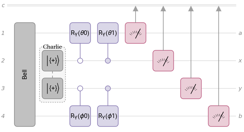
Find the measurement probabilities of the above circuit.
In[]:=
FullSimplify[#,Assumptions->{{θ0,θ1,ϕ0,ϕ1}∈Reals}]&/@qc[θ0,θ1,ϕ0,ϕ1][]["Probabilities"]
Out[]=
0000(1+Cos[θ0-ϕ0]),0001,0010(1+Cos[θ0-ϕ1]),0011,0100(1+Cos[θ1-ϕ0]),0101,0110(1+Cos[θ1-ϕ1]),0111,1000,1001(1+Cos[θ0-ϕ0]),1010,1011(1+Cos[θ0-ϕ1]),1100,1101(1+Cos[θ1-ϕ0]),1110,1111(1+Cos[θ1-ϕ1])
1
16
1
8
2
Sin
θ0-ϕ0
2
1
16
1
8
2
Sin
θ0-ϕ1
2
1
16
1
8
2
Sin
θ1-ϕ0
2
1
16
1
8
2
Sin
θ1-ϕ1
2
1
8
2
Sin
θ0-ϕ0
2
1
16
1
8
2
Sin
θ0-ϕ1
2
1
16
1
8
2
Sin
θ1-ϕ0
2
1
16
1
8
2
Sin
θ1-ϕ1
2
1
16
Given all measurement results, check which ones are winning cases.
In[]:=
(BitXor[#1,#4]==BitAnd[#2,#3])&@@@Tuples[{0,1},4]
Out[]=
{True,False,True,False,True,False,False,True,False,True,False,True,False,True,True,False}
Pick only winning cases.
In[]:=
winningCases=Pick[Values[FullSimplify[#,Assumptions->{{θ0,θ1,ϕ0,ϕ1}∈Reals}]&/@qc[θ0,θ1,ϕ0,ϕ1][]["Probabilities"]],(BitXor[#1,#4]==BitAnd[#2,#3])&@@@Tuples[{0,1},4]]
Out[]=
(1+Cos[θ0-ϕ0]),(1+Cos[θ0-ϕ1]),(1+Cos[θ1-ϕ0]),,(1+Cos[θ0-ϕ0]),(1+Cos[θ0-ϕ1]),(1+Cos[θ1-ϕ0]),
1
16
1
16
1
16
1
8
2
Sin
θ1-ϕ1
2
1
16
1
16
1
16
1
8
2
Sin
θ1-ϕ1
2
Find the probability of winning.
In[]:=
proWinning=Total[winningCases]//FullSimplify
Out[]=
1
8
Find the optimum rotation angle to win the game.
In[]:=
max=NMaximize[{proWinning,0{θ0,θ1,ϕ0,ϕ1}π},{θ0,θ1,ϕ0,ϕ1}]
Out[]=
{0.853553,{θ01.21042,θ12.78122,ϕ01.99582,ϕ10.425022}}
As one can see, with this quantum strategy, one can go beyond classical one.
Another strategy (not useful)
Another strategy (not useful)
We have the equation for winning probabilities. We would try random angles for gates of quantum circuit in this section. This section is useful in sense that even these angles must be optimized to see quantum advantage.
R
Y
Create a function which incorporates different angles in the quantum circuit after the bell circuit. We have used additional gates for this purpose.
R
y
In[]:=
quantumcirc[θ_,ϕ_]:=QuantumCircuitOperator[{"Bell",QuantumOperator[{"RY",θ},{1}],QuantumOperator[{"RY",ϕ},{2}],{1},{2}}]
In[]:=
quantumcirc[θ,ϕ]["Diagram"]
Out[]=
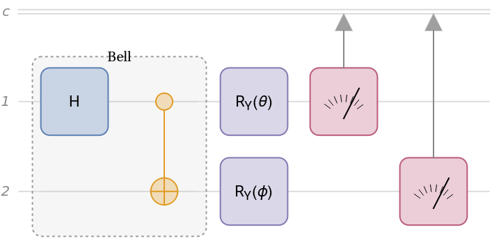
Assuming the range of both angles to be from 0 to 2π, find the probabilities associated with different combination of quantum bits.
In[]:=
$Assumptions={0<=thetaA<=2π,0<=thetaB2π};prob=KeyMap[#["Name"]&][FullSimplify/@quantumcirc[thetaA,thetaB][]["Probabilities"]]
Out[]=
{0,0}(1+Cos[thetaA-thetaB]),{0,1}(1-Cos[thetaA-thetaB]),{1,0}(1-Cos[thetaA-thetaB]),{1,1}(1+Cos[thetaA-thetaB])
1
4
1
4
1
4
1
4
Define it as probability distribution.
In[]:=
=ProbabilityDistribution[Which@@Sequence@@@Append[KeyValueMap[{{a,b}==#1,#2}&][prob],{True,0}],{a,0,∞,1},{b,0,∞,1}];
Check that the results are only 0 and 1
Check reproduces probabilities(trivial, as expected) show above.
Find the winning probabilities.
Find the maxima and angles associated in terms of π.
This is definitely equal to optimal classical strategy, therefore we need to change our strategy of choosing random angle for the optimal quantum strategy.
Initialization cells
Initialization cells
References
References
CITE THIS NOTEBOOK
CITE THIS NOTEBOOK
CHSH Game: illustrating the peculiar advantages of quantum strategies over classical ones
by Shivam Sawarn
Wolfram Community, STAFF PICKS, October 16, 2023
https://community.wolfram.com/groups/-/m/t/3036763
by Shivam Sawarn
Wolfram Community, STAFF PICKS, October 16, 2023
https://community.wolfram.com/groups/-/m/t/3036763