I have always had an interest in topology but was very interested in how quickly the multiway systems branched out as the power of the polynomials increased. Using WL and functions like Graph3D and ResourceFunction["NestGraphTagged"], we can make 3D models of directed graphs to create unique topological shape. Furthermore, we can find examine certain features of these graphs like the vertex degree or the number of loops and find similarities between these figures based on the relationships between their respective polynomial/numerical input and functions.
Basic Explanation of Multiway Systems
Basic Explanation of Multiway Systems
A multiway system can be described as taking an initial value/function and changing its state each time according to some rule(s). This included merging any states that are identical. In other words, multiway systems can have a collection of states at any step such as the figure shown below. After the first step, it is in two states (called 1 and 2). But as we progress each step, the number of states is increasing. This specific graph is using the functions n and n+1, so the number of states is growing linearly. With polynomial functions, the number of states will usually grow exponentially.
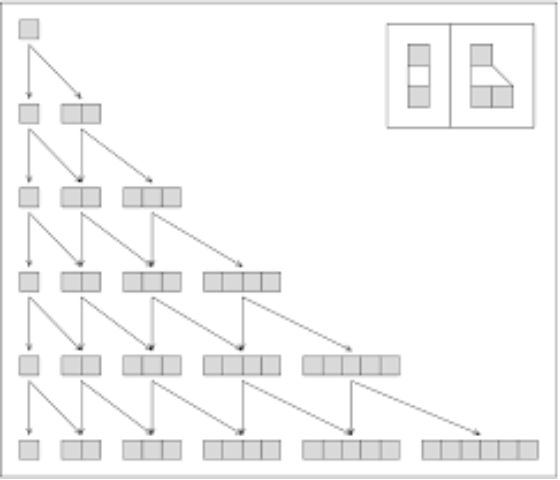
Initial Linear Computational Functions
Initial Linear Computational Functions
The first step to begin was to examine certain patterns within linear functions before preceding to polynomial functions. With pairs of functions in the form x + b, and inputs as integers, we were able to form tube-like shapes.
In[]:=
Graph3D[ResourceFunction["NestGraphTagged"][n{n+7,n+11},{0},20],VertexSize->.5,VertexStyle->Darker[,.25]]

Out[]=

Next, we create a function to manipulate the constants to observe how the graph changes.
In[]:=
Manipulate[Graph3D[ResourceFunction["NestGraphTagged"][n{n+c,n+d},{0},20],VertexSize->.5,VertexStyle->Darker[,.25]],{c,1,21,1},{d,1,21,1},SaveDefinitionsTrue]
Out[]=


Numerical Inputs w/ Polynomial Functions
Numerical Inputs w/ Polynomial Functions
Here, we created two tables: one with the functions and a second with integers. Then, we create a third table showing the pairs of functions. Now, we can visualize each of the graphs with the polynomial functions.
In[]:=
pfunctions={n^2,n^2/2,n+1,n/2,n^2+2n,n^2-2n,n^3,2n,3n+1,n-1};ninputs=Range[15];pFuncPairs=Map[(n|->#)&,Subsets[pfunctions,{2}]]
Out[]=
Functionn,,,Function[n,{,1+n}],Functionn,,,Function[n,{,2n+}],Function[n,{,-2n+}],Function[n,{,}],Function[n,{,2n}],Function[n,{,1+3n}],Function[n,{,-1+n}],Functionn,,1+n,Functionn,,,Functionn,,2n+,Functionn,,-2n+,Functionn,,,Functionn,,2n,Functionn,,1+3n,Functionn,,-1+n,Functionn,1+n,,Function[n,{1+n,2n+}],Function[n,{1+n,-2n+}],Function[n,{1+n,}],Function[n,{1+n,2n}],Function[n,{1+n,1+3n}],Function[n,{1+n,-1+n}],Functionn,,2n+,Functionn,,-2n+,Functionn,,,Functionn,,2n,Functionn,,1+3n,Functionn,,-1+n,Function[n,{2n+,-2n+}],Function[n,{2n+,}],Function[n,{2n+,2n}],Function[n,{2n+,1+3n}],Function[n,{2n+,-1+n}],Function[n,{-2n+,}],Function[n,{-2n+,2n}],Function[n,{-2n+,1+3n}],Function[n,{-2n+,-1+n}],Function[n,{,2n}],Function[n,{,1+3n}],Function[n,{,-1+n}],Function[n,{2n,1+3n}],Function[n,{2n,-1+n}],Function[n,{1+3n,-1+n}]
2
n
2
n
2
2
n
2
n
n
2
2
n
2
n
2
n
2
n
2
n
3
n
2
n
2
n
2
n
2
n
2
2
n
2
n
2
2
n
2
2
n
2
n
2
2
n
2
n
2
3
n
2
n
2
2
n
2
2
n
2
n
2
2
n
2
n
3
n
n
2
2
n
n
2
2
n
n
2
3
n
n
2
n
2
n
2
2
n
2
n
2
n
3
n
2
n
2
n
2
n
2
n
3
n
2
n
2
n
2
n
3
n
3
n
3
n
In[]:=
numInputResult=Table[ResourceFunction["NestGraphTagged"][pair,{i},6],{i,ninputs},{pair,pFuncPairs}];
In[]:=
Manipulate[numInputResult[[i,j]],{i,1,Dimensions[numInputResult][[1]],1},{j,1,Dimensions[numInputResult][[2]],1},SaveDefinitionsTrue]
Out[]=
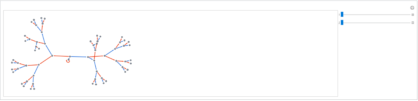
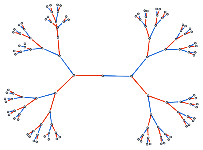
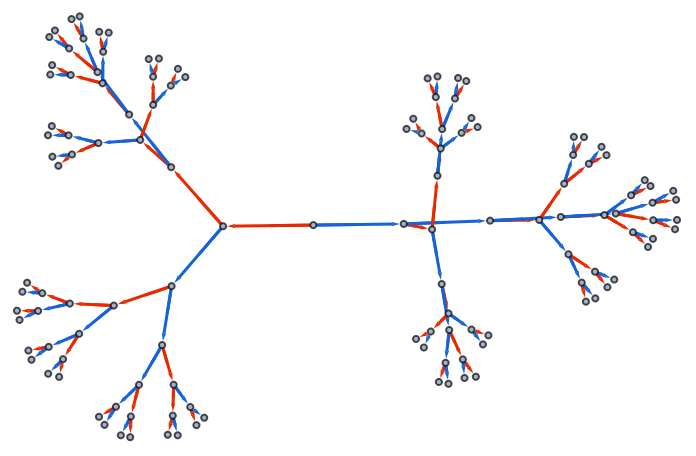
Many of these graphs seem to reflect a directed graph without loops, meaning no values repeat like the few below.
Loops Within Graphs
Loops Within Graphs
To determine this, I used the function LoopFreeGraphQ. From there, I converted the variables to 0 and 1 and graphed them to observe how the frequency of loops changes as the graphs become more complex.
In[]:=
loops=Flatten[Table[LoopFreeGraphQ[numInputResult[[i,j]]],{i,Length[numInputResult]},{j,Length[numInputResult]}]];
In[]:=
BarChart[Table[If[loops[[i]],1,0],{i,Dimensions[loops][[1]]}],AxesLabel{None,Style["Occurence of Loops",10]}]
Out[]=
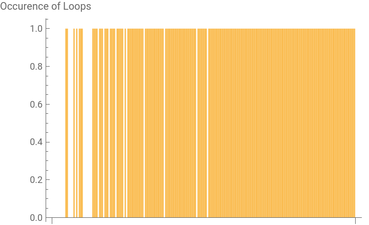
Additionally, I made a function to find the degree of each vertex within each graph. VertexDegree is a function that counts how many arrows are connected to the one vertex. Using this function, I created a bar chart to see the frequency of vertex degree values across the graphs.
Applications to More Complex Polynomials
Applications to More Complex Polynomials
Given the previous functions, we were able to make fairly simple graphs that could easily be traced. However, this time, we included complex functions like derivatives and integrals.
Polynomial Inputs w/ Polynomial Functions
Polynomial Inputs w/ Polynomial Functions
When using polynomial inputs for polynomial functions, the power of the functions will keep increasing since you are applying a polynomial function to a polynomial input. This will lead to a long runtime and take up a lot of storage, causing the program to crash. Instead, we must use polynomials functions that will reduce the power such as the derivative function. Additionally, we can multiply functions by linear functions to create polynomials. Specifically, we will be examining how quickly the counts of vertices and edges grow as well as how the complexity of graphs change based on different functions.
To begin, I started with a fairly simple input and only two complex functions, the derivative as well as multiplying 'x' and the function. Then, I ran the code for ten iterations to see the progression of the graph's complexity.
To begin, I started with a fairly simple input and only two complex functions, the derivative as well as multiplying 'x' and the function. Then, I ran the code for ten iterations to see the progression of the graph's complexity.
To plot the counts of vertices and edges, we need to count them for each individual graph and find a best fit line to demonstrate how the numbers grow.
To investigate how changes in different parts of the equation will affect the exponential equation, I first changed the constant.
When comparing these functions to the ones shown first, we see that the vertex modeling equation and the edge modeling equation is exactly the same, meaning the constants have no significant effect on the branching of the graph. Further examination also shows that adding a coefficient to the variable 'x' also does not change the best fit curve.
Future Research
Future Research
For future research in multicomputational polynomials, I could pursue an interest in different quantitative aspects such as the short path between the two farthest points and see how this tends to change as the number of iterations increases. Additionally, I could also pursue relationships between the multiway graphs, including reductions and simplification.
Citations
Citations