Black box optimization is a branch of optimization that deals with derivative-free functions. This means that the function’s derivative is unknown because finding it is impossible or impractical. Different methods like Random Search, Grid Search, and some Heuristics are used to solve these optimization problems. One recent approach used in this area is the Mesh Adaptive Direct Search (MADS) method. This paper aims to explain the creation of a function in Mathematica that runs MADS algorithm and returns a minimum. This function has been successfully implemented, throwing good results in global minima search. Nevertheless, using it in functions with many local minima is not suggested because it might get trapped in one of these minimums. Also, in the examples, there are functions with problematic derivatives that are successfully solved. The function was named MadsOptimizer, and it takes two parameters. The first parameter is the objective function, and the second is a list of the variables. Given the positive results of the MADS implementation, the code can be turned into a built-in Wolfram Language function that can be used in different areas. MADS is widely used for parameter fit and other problems involving simulations and experiments. Also, this project suggests an addition to the MadsOptimizer function, increasing the chances of getting the global minima. This paper grasps some of the theory behind the method, shows some results using different functions, and uses a visual representation to show the path taken by the algorithm.
Theory:
Theory:
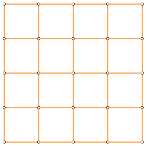
The main point of this paper is to show the results of the Mesh Adaptive Direct Search (MADS) method and why it is a good tool. However, to understand the significance of MADS, it is beneficial to have a basic understanding of its theory. MADS can be seen as a generalization of the Generalized Pattern Search (GPS) optimization method, building upon its principles and introducing new concepts for improved performance. One of the key concepts in the MADS algorithm is the notion of a mesh. In optimization, the mesh refers to the grid or lattice structure that covers the search space. It divides the domain into smaller regions, allowing for a systematic exploration of the parameter space. The mesh helps guide the search by determining the regions to be explored and the precision with which the search is conducted. By adapting the mesh dynamically based on the search progress, MADS can effectively navigate complex and irregular landscapes.
Out[]=
Mesh |
Mesh and Frame |
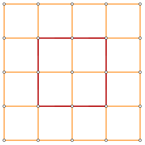
Another essential component of the MADS algorithm is the “frame.” The frame represents a subset of the mesh, defining the region where the search is currently focused. It acts as a window that constrains the search to a specific part of the parameter space. By adjusting the frame during the optimization process, MADS can adaptively zoom in or out of different areas, allocating computational resources efficiently and directing the search towards promising regions. The “poll set” is another crucial element of the MADS algorithm. It consists of a collection of trial points carefully selected within the frame, which are used to evaluate the objective function. These trial points serve as candidates for potential improvement, allowing the algorithm to make informed decisions about which regions of the parameter space to explore further. The poll set plays a pivotal role in balancing exploration and exploitation, enabling MADS to refine the search and converge toward an optimal solution efficiently. Understanding the interplay between these three objects—, the mesh, the frame, and the poll set—provides insights into the inner workings of the MADS algorithm. While the demonstration of convergence is beyond the scope of this paper, the utilization of these concepts in MADS enables it to achieve improved optimization performance in a variety of real-world problems.
The Code:
The Code:
The main idea behind MADS is to iteratively build and adapt a mesh of trial points in the search space based on the information obtained from function evaluations. The algorithm aims to explore the search space efficiently, avoiding unnecessary function evaluations in regions where the function is unlikely to improve.
The MADS algorithm can be divided into five main steps, so in this section, those steps will be explained through the implementation in Wolfram Language. The first of the steps is the initialization, which initializes the algorithm parameters, such as the stopping tolerance, initial frame size parameter, and other control parameters like setting the iterator to zero. The function requires the exprn_ and vars_ parameters, which are the function to optimize and its variables, respectively. The user can manipulate the rest of the options if it helps to address a specific problem.
The MADS algorithm can be divided into five main steps, so in this section, those steps will be explained through the implementation in Wolfram Language. The first of the steps is the initialization, which initializes the algorithm parameters, such as the stopping tolerance, initial frame size parameter, and other control parameters like setting the iterator to zero. The function requires the exprn_ and vars_ parameters, which are the function to optimize and its variables, respectively. The user can manipulate the rest of the options if it helps to address a specific problem.
Options[MadsOptimizer]={iterations->10000,meshAdjustment->0.9,stopTolerance->10^-60,initialFrameSize->1};MadsOptimizer[exprn_,vars_,OptionsPattern[]]:=Module[{nDimension=Length[vars],kStop=OptionValue[iterations],T=OptionValue[meshAdjustment],tolerance=OptionValue[stopTolerance],DeltaFrame=OptionValue[initialFrameSize],kStart=1,deltaMesh},...]
The second step is simple: update the mesh size parameter, which depends on the frame size parameters. Here it is defined as the minimum value between the frame and the square of the frame, but it can be defined in other ways.
deltaMeshUpdate=Min[{#,#^2}]&
The third step randomly picks a point from the mesh and makes a comparison with the current best point. If the search is successful, the termination step is executed. If the search fails, then the poll step is executed. In this step, the algorithm generates polling points by combining the direction with mesh sizes associated with each direction. Polling points are trial points that will be evaluated to determine if there is an improvement over the current best solution. Moreover, this polling set is an asymptotically dense set of directions, which ensures that the algorithm can approach the optimal solution as the number of iterations or function evaluations tends to infinity. This is necessary to use the Householder matrix and some other operations involving the mesh and frame size parameters. This is a way of picking one direction among the set of directions the frame offers.
HouseholderMatrix[vector_]:=IdentityMatrix[Length[vector]]-2Transpose[{vector}].{vector}/(vector.vector)RandomPollStep[nDimension_Integer,DeltaFrame_]:=Module[ vector=Normalize[RandomReal[1,nDimension]], deltaMesh1=Min[deltaFrame^2,deltaFrame], Hmat, Bset, Dset, Hmat=HouseholderMatrix[vector]; Bset=(Round[(deltaFrame/deltaMesh)*(#/Norm[#,Infinity])]&)/@Transpose[Hmat]; Dset=Transpose@Join[Bset,-Bset]; Return[Transpose[Dset][[RandomInteger[{1,2*nDimension}]]]] ]
The objective function is evaluated at a randomly selected polling point to obtain the corresponding function value. Then, the function value is compared with the current best solution to determine if any improvement is found. If any polling point yields a better solution, the current best solution is accordingly updated. The best solution is typically the point with the lowest function value.
currentPoint=(bestPoint+deltaMesh*RandomPollStep[nDimension,DeltaFrame])
Based on the evaluation results of the polling points, adapt the frame sizes associated with each search direction. The frame sizes control the density of trial points along each direction. If a direction leads to improved solutions, the frame size in that direction may be decreased to focus the search. Conversely, if a direction is unproductive, the frame size may be increased to reduce the sampling density.
If[ObjectiveFunction@@currentPoint<ObjectiveFunction@@bestPoint,(*IfTrue,updatethebestpointandexpandtheframesize*)bestPoint=currentPoint;DeltaFrame=DeltaFrame/T,(*IfFalse,makesmallertheframe*)DeltaFrame=DeltaFrame*T]
The final step is to check if the termination criteria are met. These criteria can be based on the number of iterations, the established tolerance, or a specific target objective value. If the termination criteria are satisfied, stop the algorithm and return the current best solution as the approximate optimal solution. In this implementation, the two termination criteria are iterations and tolerance.
If[DeltaFrame>=tolerance,kStart++,Return[{N[ObjectiveFunction@@bestPoint],N[bestPoint]}]]
In addition to the MADS algorithm, a piece of code was added. This extension is a function called MoxOptimizer and, like MadsOptimizer, has the objective function and respective variables as required parameters. The main idea of this extension is to run the MADS algorithm several times. The objective is to initialize the search with different random vectors and then pick the best of the MADS outcomes, which increases the probability of getting the correct answer. The following example shows the difference between MadsOptimizer and MoxOptimizer.
In[]:=
MadsOptimizer[-Cos[x]*Cos[y]*^(-(x-π)^2-(y-π)^2),{x,y}]
Out[]=
MadsOptimizer-Cos[x]Cos[y],{x,y}
--
2
(-π+x)
2
(-π+y)
In[]:=
MoxOptimizer[-Cos[x]*Cos[y]*^(-(x-π)^2-(y-π)^2),{x,y}]
Out[]=
MoxOptimizer-Cos[x]Cos[y],{x,y}
--
2
(-π+x)
2
(-π+y)
Notice how the MoxOptimizer function is slower than the MadsOptimizer; however, MoxOptimizer has more chance to give the correct global minima. This improvement is not rooted in the structure of the second function; instead, the improvement comes because of the change of the initial vectors with each iteration. Also, by augmenting the repetitions option, both running time and the chance of getting the correct answer increase.
In[]:=
MoxOptimizer[-Cos[x]*Cos[y]*^(-(x-π)^2-(y-π)^2),{x,y},repetitions->12]
Out[]=
MoxOptimizer-Cos[x]Cos[y],{x,y},repetitions12
--
2
(-π+x)
2
(-π+y)
In[]:=
MoxOptimizer[-Cos[x]*Cos[y]*^(-(x-π)^2-(y-π)^2),{x,y},repetitions->2]
Out[]=
MoxOptimizer-Cos[x]Cos[y],{x,y},repetitions2
--
2
(-π+x)
2
(-π+y)
Testing:
Testing:
After several tests, the MadsOptimizer and MoxOptimizer functions improved over the NMinimize in specific cases. One example is the function previously used, which is known as the Easom function and is defined as: The next cell contains the result of evaluating the Easom function in NMinimize.
f(x,y)-cos(x)·cos(y)·
--
2
(x-π)
2
(y-π)
e
In[]:=
NMinimize[-Cos[x]*Cos[y]*^(-(x-π)^2-(y-π)^2),{x,y}]
Out[]=
{-0.0000811022,{x1.305,y1.305}}
In contrast, if MadsOptimizer is used, there is a chance of getting the correct answer which is f(π,π)==-1. In addition to this, if the MoxOptimizer is evaluated, the chance of getting the correct answer is high.
In[]:=
MadsOptimizer[-Cos[x]*Cos[y]*^(-(x-π)^2-(y-π)^2),{x,y}]
Out[]=
MadsOptimizer-Cos[x]Cos[y],{x,y}
--
2
(-π+x)
2
(-π+y)
In[]:=
MoxOptimizer[-Cos[x]*Cos[y]*^(-(x-π)^2-(y-π)^2),{x,y}]
Out[]=
MoxOptimizer-Cos[x]Cos[y],{x,y}
--
2
(-π+x)
2
(-π+y)
The graph below is a representation of how MadsOptimizer finds the global minima.
Out[]=
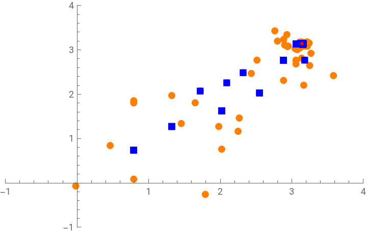


The red dot represents the coordinates of the minima, the blue squares are the best points found, and the orange dots are all the points’ progression. Here, the algorithm starts searching points in the mesh and gradually approaches the global minimum. Nevertheless, it is essential to be aware that this behavior may lead to local minima in which the algorithm might get trapped.
This other visualization represents the path of the best points connected by straight blue lines. The rest of this notebook is dedicated to show a few examples of some functions evaluated in NMinimize, MadsOptimizer and MoxOptimizer respectively.
Here the NMinimize does not arrive at the correct answer. On the other hand, MadsOptimizer does arrive at the correct global minima very often, while MoxOptimizer gets the minima most of the time.
The second example shows how MadsOptimizer and NMinimize arrive at the same minima, though, MoxOptimizer found a better answer. MoxOptimizer does not always arrive at the same coordinate and might sometimes arrive at the same point that the other two functions. Finally, the third example shows that the three functions arrived at the same minima. One aspect of the NMinimize is that it always has the same outcome, while MadsOptimizer and MoxOptimizer may give different answers for the same function. Nevertheless, MoxOptimizer is usually stable in its outputs because of the repetitions.
MadsOptimizer
MadsOptimizer
MoxOptimizer
MoxOptimizer
Concluding Remarks
Concluding Remarks
In this project two functions were developed. The first function is MadsOptimizer, and its code is based on the Mesh Adaptive Direct Search (MADS) algorithm. This method is helpful in Black Box optimization, solving derivative-free functions and other functions with problematic derivatives. It can be applied to fields like Material Science, Energy, and Computer Science. One interesting approach is to optimize the hyperparameters in Machine Learning. Because of the time such an application may take, it was left for future research work. The second function developed depends on the first, a straightforward and logical extension. The MoxOptimizer function will execute the MADS algorithm several times, allowing different starting vectors to help find other solutions. These solutions are stacked in a list in increasing order for the evaluation, and finally, the first element is selected as the solution. Summing up,the algorithm was implemented as a function in Wolfram Language with the name MadsOptimizer. In addition, another function (MoxOptimizer) was created to improve the search of the global minima. The MadsOptimizer function showed some improvement in finding global minima in specific functions when compared with the functions NMinimize.
Keywords
Keywords
◼
Blackbox
◼
MADS
◼
Householder matrix
◼
Global minima
Acknowledgment
Acknowledgment
I want to thank God and my family, who gave everything. I am also grateful to my mentor Sotiris who helped me from the project selection until the culmination. I want to thank Christian Pasquel for the guidance since week zero. I thank Robert Nachbar for his availability and great Wolfram Language introduction lectures. I am also thankful to Joshua Pedro, Fez Zaman, Mark Greenberg, Swastik Banerjee, John McNally, Daniel Sanchez, and, in general, all available mentors. Finally, I want to thank Mads Bahrami, Yi Yin, Stephanie Bowyer, and Ahmed Elbanna for their patience and exceptional guidance through these three weeks. Finally, I am profoundly thankful to Stephen Wolfram for making this fantastic learning experience possible.
References
References
◼
Audet, Charles, and Warren Hare. Derivative-Free and Blackbox Optimization. Springer, 2 Dec. 2017.
◼
Charles, Audet, and Denis J. Mesh Adaptive Direct Search Algorithm for Constrained Optimization. 1 Jan. 2006, www.researchgate.net/publication/220133585_Mesh_Adaptive_Direct_Search_Algorithms_for_Constrained_Optimization.
◼
Alarie, Stéphane, et al. “Two Decades of Blackbox Optimization Applications.” EURO Journal on Computational Optimization, vol. 9, 1 Jan. 2021, p. 100011, www.sciencedirect.com/science/article/pii/S2192440621001386#:~:text=Blackbox%20optimization%20(BBO)%20considers%20the, https://doi.org/10.1016/j.ejco.2021.100011. Accessed 3 Mar. 2023.
◼
Audet, Charles, and Michael Kokkolaras. “Blackbox and Derivative-Free Optimization: Theory, Algorithms and Applications.” Optimization and Engineering, vol. 17, no. 1, 1 Feb. 2016, pp. 1–2, https://doi.org/10.1007/s11081-016-9307-4.
CITE THIS NOTEBOOK
CITE THIS NOTEBOOK
Black box optimization: the mesh adaptive direct search (MADS) algorithm
by Moises Gonzalez
Wolfram Community, STAFF PICKS, July 12, 2023
https://community.wolfram.com/groups/-/m/t/2958734
by Moises Gonzalez
Wolfram Community, STAFF PICKS, July 12, 2023
https://community.wolfram.com/groups/-/m/t/2958734