Block cellular automaton (BCA) provides a natural framework for constructing reversible cellular automata. For two binary cells per block, the reversible local rules are the 24 permutations in . Replacing these permutation rules with general two-qubit unitaries in yields a partitioned quantum cellular automaton (PQCA), whose global states evolve in a -dimensional Hilbert space for qubits. In this project, we study the quantum thickening of the classical BCA rule space by continuously interpolating between adjacent rules through paths in . Although the endpoints of each path are classical permutation rules, the intermediate unitaries can generate nontrivial superposition and many-body entanglement in the resulting QCA dynamics. We compare these coherent unitary paths with incoherent mixed-unitary channels that probabilistically alternate between the same classical endpoints, asking whether the intermediate quantum behavior can be reproduced by classical endpoint averaging. Our results show that the coherent paths generate information dynamics that are generally not captured by the corresponding incoherent mixtures, demonstrating that the continuous interior of contains genuinely quantum structure beyond the discrete classical rule space .
S
4
U(4)
n
2
n
S
4
U(4)
U(4)
S
4
Introduction
Introduction
Classical Reversible Block Cellular Automata
Classical Reversible Block Cellular Automata
A classical block cellular automaton (BCA) applies a deterministic rule to fixed-size blocks of cells. For two-bit binary blocks, the rule maps each block to another block of the same size. To allow information to propagate across block boundaries, BCAs commonly use Margolus partitioning, in which the two-cell groupings are shifted on alternating time steps. We focus on reversible BCAs, whose local rules must be permutations of the four possible two-bit configurations. Because this rule space is small, only limited behavior is expected at the local level.
Implementation: ruleGraphic, blockCA, plotCA, visualizeMarg
Implementation: ruleGraphic, blockCA, plotCA, visualizeMarg
Application:
Application:
In[]:=
rule=reversibleRules[[3]];Print["Rule:"]ruleGraphic[rule]
Rule:
Out[]=
In[]:=
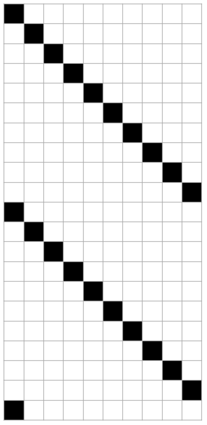
init={1,0,0,0,0,0,0,0,0,0};phase=0;evolution=blockCA[rule,init,phase,20];visualizeMarg[evolution]
Margolus Neighborhoods
t = 0 phase = 0 blocks = {{1,2},{3,4},{5,6},{7,8},{9,10}}
t = 1 phase = 1 blocks = {{2,3},{4,5},{6,7},{8,9},{10,1}}
...
In[]:=
plotCA[evolution]
Out[]=
Quantum Cellular Automata
Quantum Cellular Automata
One example of a quantum cellular automaton is the block partitioned quantum cellular automaton (PQCA). It generalizes reversible block cellular automata by replacing classical permutation rules with two-qubit unitaries in and binary cell states with quantum states in . This construction satisfies the axioms of quantum evolution while providing a simple framework for simulating quantum systems. PQCA are also computationally universal, they can simulate any quantum algorithm with at most a linear slowdown. They therefore offer a simple but powerful model for constructing and studying quantum dynamics.
The main difficulty is that quantum cellular automata are extremely resource-intensive to simulate classically for arbitrary states and unitaries. For a system of qubits, the state vector contains complex amplitudes, so the required memory grows exponentially with system size. This rapid expansion of the Hilbert space severely limits the size and duration of simulations that can be performed using classical computers.
U(4)
{0,1}
2
The main difficulty is that quantum cellular automata are extremely resource-intensive to simulate classically for arbitrary states and unitaries. For a system of
n
n
2
In[]:=
Table[<|"Qubits"->n,"State Vector Dimension"->2^n|>,{n,2,14,2}]//Dataset
Out[]=
An efficient PQCA method is therefore mandatory. For this project, we developed an efficient PQCA paclet called DenizYoldas/QuantumBlockCellularAutomata.
Install Paclet and Distribute Across Kernels:
Install Paclet and Distribute Across Kernels:
Application:
Application:
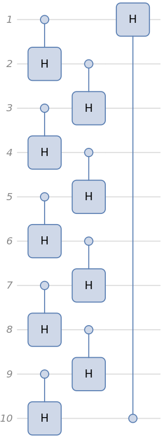
This paclet provides a function called , which accepts an initial layer of quantum states, a unitary evolution rule, the number of full Margolus cycles to apply, and an optional phase argument that determines the partitioning. The initial layer may be specified as a classical bitstring, a normalized numerical state vector, or a object. The evolution rule may be given as either a or a numerical 4x4 unitary matrix. Each full time step consists of both the even and odd Margolus partitions. The function uses ring boundary conditions, as in reversible block cellular automata. This partitioning scheme is illustrated in the full Margolus block circuit diagram below.
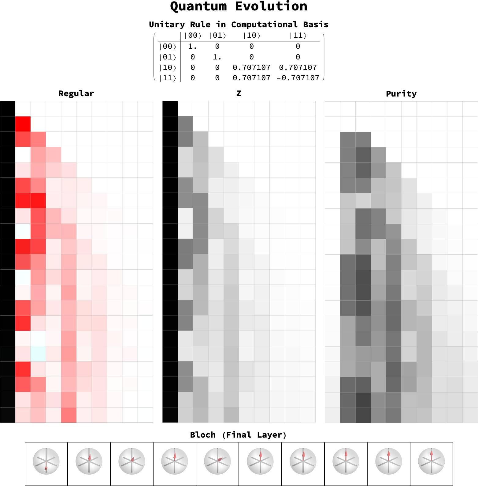
The paclet also includes, which provides several visualization options based on the reduced density matrix of each cell in a quantum layer. Further implementation details are available in the paclet documentation.
QuantumCA
QuantumState
QuantumOperator
The paclet also includes
PlotQuantumCA
In[]:=
evo=QuantumCA[{1,0,0,0,0,0,0,0,0,0},QuantumOperator["CH"],10];Dataset[evo,MaxItems->{2}]
Out[]=

Plot the full Margolus circuit:
In[]:=
evo["Circuit"]["Diagram"]
Out[]=
Plot the evolution (see appendix for color function descriptions):
In[]:=
PlotQuantumCA[evo,"Views"->{"Regular","Z","Purity","Bloch"}]
Out[]=
Evolve superposition or entangled input states:
Classical Rule Geometry
Classical Rule Geometry
The 24 Permutation Rules
The 24 Permutation Rules
Evolutions for all 24 permutation rules of S4:
Graph of maximal generating set:
Graph of minimal generating set:
Graph of minimal self-inverse generating set:
Quantum Thickening: Coherent Unitary Interpolation
Quantum Thickening: Coherent Unitary Interpolation
Constructing the Continuous Unitary Path
Constructing the Continuous Unitary Path
Application:
Application:
An example unitary path between I and CX:
Information Measures for the Coherent Channel
Information Measures for the Coherent Channel
Application:
Application:
Metrics for the I to CX path above for theta ~ 0.5:
Consistency checks:
Application:
Application:
Metric heat map for full path (plots are compressed from theta axis):
Information Space Analysis on Cayley Graph
Information Space Analysis on Cayley Graph
Undirected graph of minimal self-inverse generating set:
Application:
Application:
Calculate quantumness of each edge (intensive parallel simulation required):
Calculate mean entanglement entropy per edge and construct the Cayley Graph:
Here we see some interesting results, while most of the edges create high entanglement, some of them stay quite low.
Edge weights histogram, it is evident that some vertices create almost none bi-partite entanglement:
The low entangling coherent path between vertices 3 and 13. The cells stay locally pure and mostly local superpositions form during the path:
The high entangling coherent path between vertices 15 and 16. The cells get locally mixed and local Bloch vectors shrink to towards origin:
Classical View: Incoherent Endpoint Averaging
Classical View: Incoherent Endpoint Averaging
Constructing the Stochastic Classical Path
Constructing the Stochastic Classical Path
Application:
Application:
An example incoherent path between I and CX (plot shows the Z measurements for each cell):
Information Measures for the Incoherent Channel
Information Measures for the Incoherent Channel
Application:
Application:
Metrics for the incoherent I to CX path above for theta ~ 0.5:
Consistency checks:
Application:
Application:
The von Neumann entropy heat map for full path:
Information Space Analysis on Cayley Graph
Information Space Analysis on Cayley Graph
The von Neumann entropy of each edge (extremely intensive parallel simulation required):
Calculate mean von Neumann entropy per edge and construct the Cayley Graph:
Here we also see some interesting results, while most of the edges create high mixing, some of them stay quite low.
Edge weights histogram, some vertices create low mixing although none of them approach zero:
The low mixing incoherent path between vertices 5 and 11. The global state stays mostly pure:
The high mixing incoherent path between vertices 15 and 16. The global state get mixed:
Comparison Between Coherent and Incoherent Paths
Comparison Between Coherent and Incoherent Paths
Comparison Metric
Comparison Metric
Results on Cayley Graph
Results on Cayley Graph
Mean variation distance calculated for each edge:
The results are interesting, but we should also examine the edge-weight histogram, since the edge thicknesses are min–max normalized.
Edge weights histogram, all values are higher than 0.5, and most of them are close to the max value of 1:
The three Cayley graph results are summarized below:
Conclusion
Conclusion
Acknowledgements
Acknowledgements
I would like to thank my advisor, Nik Murzin, for his support and mentorship throughout this project. I am also grateful to Stephen Wolfram for his guidance in shaping the initial research direction. Finally, I thank Xerxes Arsiwalla and the other WSRI26 program mentors for their teaching, support, and mentorship.
References
References
Software and Documentation
Yoldas, Deniz. *QuantumBlockCellularAutomata*. Wolfram Community Paclet Repository.
Wolfram Community
Stocke, Joseph. “Exploring Quantum Cellular Automata with the Wolfram Quantum Paclet.” Wolfram Community, 2022.
Books
Wolfram, Stephen. *A New Kind of Science*. Wolfram Media, 2002.
Yoldas, Deniz. *QuantumBlockCellularAutomata*. Wolfram Community Paclet Repository.
Wolfram Community
Stocke, Joseph. “Exploring Quantum Cellular Automata with the Wolfram Quantum Paclet.” Wolfram Community, 2022.
Books
Wolfram, Stephen. *A New Kind of Science*. Wolfram Media, 2002.
Nielsen, Michael A., and Isaac L. Chuang. *Quantum Computation and Quantum Information*. 10th anniversary ed., Cambridge University Press, 2010.
Papers
Arrighi, Pablo. “An Overview of Quantum Cellular Automata.” ArXiv.org, 6 Sept. 2019, https://arxiv.org/abs/1904.12956.
Papers
Arrighi, Pablo. “An Overview of Quantum Cellular Automata.” ArXiv.org, 6 Sept. 2019, https://arxiv.org/abs/1904.12956.
Schumacher, B., and R. F. Werner. “Reversible Quantum Cellular Automata.” ArXiv.org, 28 May 2004, https://arxiv.org/abs/quant-ph/0405174.
Watrous, John. “On One-Dimensional Quantum Cellular Automata.” *Proceedings of the 36th Annual Symposium on Foundations of Computer Science*, IEEE Computer Society, 1995, pp. 528–537.
AI Disclosure
AI Disclosure
The following generative AI tools were used in this project: OpenAI ChatGPT 5.5 and Wolfram Notebook Assistant. They were used for code debugging and brainstorming. All code and written content were reviewed, understood, and approved by the author.
CITE THIS NOTEBOOK
CITE THIS NOTEBOOK
Quantum Thickening of Reversible Block Cellular Automata: Analyzing Paths from S4 to U(4)
by Deniz Yoldas
Wolfram Community, STAFF PICKS, July 16, 2026
https://community.wolfram.com/groups/-/m/t/3763192
by Deniz Yoldas
Wolfram Community, STAFF PICKS, July 16, 2026
https://community.wolfram.com/groups/-/m/t/3763192