This review of the paper Jiřı Jına, Pavel Trojovský, “On Permanents of Some Tridiagonal Matrices Connected with Fibonacci Numbers”, International Journal of Pure and Applied Mathematics Volume 88 No. 4 (2013), 569-575, http://dx.doi.org/10.12732/ijpam.v88i4.11 explores the intriguing intersection between linear algebra and number theory by examining specific tridiagonal matrices whose permanents correspond to terms in the Fibonacci sequence . This connection highlights a deep structural relationship between matrix theory and well - known number sequences, offering fresh insights into the combinatorial and algebraic properties of these matrices . This essay reviews the key concepts, findings, and mathematical derivations presented in the paper and includes a computational code section to generate these matrices and verify their unique Fibonacci - related properties.
Keywords: tridiagonal matrix, permanent, Fibonacci sequence, recurrence relation, Toeplitz matrix, characteristic equation
Introduction
Introduction
Essential concepts
Essential concepts
In understanding the connection between Fibonacci numbers and tridiagonal matrices, several mathematical properties, identities, and visual representations of Fibonacci numbers play a key role.
◼
Cassini’s Identity: A classical property of Fibonacci numbers, showing a distinct relationship between consecutive terms:
F
n-1
F
n+1
2
F
n
n
(-1)
In[]:=
Cassini[n_]:=Fibonacci[n-1]*Fibonacci[n+1]-
2
Fibonacci[n]
(*yields1forasampleofevennumbers*)Cassini[Table[num,{num,0,10,2}]](*yields-1forasampleofoddnumbers*)Cassini[Table[num,{num,1,10,2}]]
Out[]=
{1,1,1,1,1,1}
Out[]=
{-1,-1,-1,-1,-1}
◼
Binet’s Formula: An explicit formula to find the n-th Fibonacci number. It relies on the roots of the characteristic equation -x-1=0, i.e.
2
x
In[]:=
Solve[-x-1==0,x]
2
x
Out[]=
x(1-(1+
1
2
5
),x1
2
5
)The solutions are the golden ratio and its conjugate . Hence, the formula is:
φ=
1+
5
2
ψ=
1-
5
2
F
n
n
φ
n
ψ
5
In[]:=
φ=;ψ=;Binet[n_]:=-
1+
5
2
1-
5
2
n
φ
n
ψ
5
Binet[15]//N(*Evaluationgfor15*)Fibonacci[15](*Evaluationgfor15*)
Out[]=
610.
Out[]=
610
◼
The Golden Ratio: The ratio between successive Fibonacci numbers and as . This proportion (also known as the Divine proportion, Golden mean, or Golden section) approaches to the golden ratio φ as approaches infinity.
F
n
F
n-1
F
n
F
n-1
n
n∞
F
n
F
n-1
In[]:=
GoldenRatio//N
Out[]=
1.61803
If we attempt to aproximate for a large number , it fails to reach the Golden Ratio.
p
In[]:=
p=100;==GoldenRatio
Fibonacci[p]
Fibonacci[p-1]
Out[]=
False
But, for a sufficient large number :
z
In[]:=
z∞
Fibonacci[z]
Fibonacci[z-1]
Out[]=
True
◼
The Fibonacci Q-matrix: A matrix used to compute Fibonacci numbers efficiently through matrix exponentiation. Defined as:
2×2
Q=
1 | 1 |
1 | 0 |
In[]:=
(matrixQ={{1,1},{1,0}})//MatrixForm
Out[]//MatrixForm=
1 | 1 |
1 | 0 |
the matrix power has the property that:
n
𝑄
n
Q
F n+1 | F n |
F n | F n-1 |
In[]:=
n=6;(MatrixPower[matrixQ,n])//MatrixForm
Out[]//MatrixForm=
13 | 8 |
8 | 5 |
In[]:=
n=6;Print["For n=",n]Print[" element: ",Part[MatrixPower[matrixQ,n],1,1]](**)Print["Fibonacci n+1 term: ",Fibonacci[n+1]]Part[MatrixPower[matrixQ,n],1,1]==Fibonacci[n+1]Print["\n element: ",Part[MatrixPower[matrixQ,n],1,2]](**)Print["Fibonacci n term: ",Fibonacci[n]]Part[MatrixPower[matrixQ,n],1,2]==Fibonacci[n]Print["\n element: ",Part[MatrixPower[matrixQ,n],2,1]](**)Print["Fibonacci n term: ",Fibonacci[n]]Part[MatrixPower[matrixQ,n],2,1]==Fibonacci[n]Print["\n element: ",Part[MatrixPower[matrixQ,n],2,2]](**)Print["Fibonacci n-1 term: ",Fibonacci[n-1]]Part[MatrixPower[matrixQ,n],2,2]==Fibonacci[n-1]
n
q
11
n
Q
11
n
q
12
n
Q
12
n
q
21
n
Q
21
n
q
22
n
Q
22
For n=6
n
q
11
Fibonacci n+1 term: 13
Out[]=
True
element: 8
n
q
12
Fibonacci n term: 8
Out[]=
True
element: 8
n
q
21
Fibonacci n term: 8
Out[]=
True
element: 5
n
q
22
Fibonacci n-1 term: 5
Out[]=
True
◼
Sum of Fibonacci Numbers: The sum of the first Fibonacci numbers can be described by the following identity:
n
n
∑
k=0
F
k
F
n+2
n
∑
k=0
Out[]=
True
◼
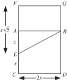
The Golden Rectangle: A golden rectangle is a rectangle whose side lengths are in the golden ratio . If a square is removed from a golden rectangle, the remaining rectangle is also a golden rectangle.
φ
◼
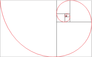
The Golden Spiral: The golden spiral is a logarithmic spiral that grows outward by a factor of for each quarter turn. It can be constructed by drawing quarter arcs within a golden rectangle and recursively removing squares.
φ
◼
The Golden Angle: The golden angle is derived from dividing a circle according to the golden ratio. It is approximately and arises in phyllotaxis, the arrangement of leaves, seeds, and other plant parts around a stem.
137.5°
3601-=360(2-φ)==180(3-
1
φ
360
2
φ
5
)◼
Fibonacci Numbers in Nature: The Fibonacci numbers are sometimes called Pine Cone Numbers (Pappas 1989, p. 224). The role of the Fibonacci numbers in botany is sometimes called Ludwig’s law (Szymkiewicz 1928; Wells 1986, p. 66; Steinhaus 1999, p. 299).
◼
Continued Fractions: Provide a way to express numbers as sequences of integer quotients. Continued fractions are useful for approximations in number theory and for revealing number patterns with a high degree of regularity.
The golden ratio φ has a particularly simple continued fraction representation:
◼
Recurrence Relation: An equation that recursively defines a sequence.
◼
Toeplitz Matrix: A matrix where each descending diagonal from left to right is constant.
◼
Characteristic Equation: An equation that defines the eigenvalues of a matrix.
◼
Symmetric Group: A group consisting of all permutations of a finite set.
◼
Laplace Expansion: A method for calculating the determinant of a matrix.
Mathematical Concepts and Properties Related to Fibonacci Numbers
Mathematical Concepts and Properties Related to Fibonacci Numbers
Tridiagonal Matrix
Tridiagonal Matrix
◼
All other entries are zero.
In this paper, the authors examine several tridiagonal matrices with specific entries, showing how their permanents yield Fibonacci numbers.
Permanent of a Matrix
Permanent of a Matrix
where σ represents all permutations of the set {1, 2, …, 𝑛}. Unlike determinants, permanents are generally more computationally intensive due to the absence of sign alternation. A matrix and its transpose have the same permanent.
(*Python code for the Permanent*)
!pip install more-itertools
from itertools import permutations
def permanent(matrix):
"""
Calculate the permanent of a square matrix.
"""
n = len(matrix)
if n == 0:
return 1
total = 0
for perm in permutations(range(n)):
term = 1
for i, j in enumerate(perm):
term *= matrix[i][j]
total += term
return total
result = permanent(matrix_A(6))
print(result) # Output: 13
print(result) # Output: 13
The Fibonacci Sequence and Matrix Permanents
The Fibonacci Sequence and Matrix Permanents
The Fibonacci sequence is a series where each term is the sum of the previous two terms, starting with 0 and 1. Mathematically, it is defined by:
The paper finds that for certain structured tridiagonal matrices, the permanent equals a Fibonacci number, demonstrating a unique structural property in these matrices.
Main Results
Main Results
The paper examines three main types of matrices, each with a permanent linked to Fibonacci numbers:
A tridiagonal matrix with 1s on the main and adjacent diagonals.
Code in python.
import numpy as np
n=6
n=6
In[]:=
def matrix_A(n):
matrix = [[0 for x in range(n)] for y in range(n)]
for i in range(n):
matrix[i][i] = 1 # Main diagonal
if i < n-1:
matrix[i][i+1] = 1 # Upper diagonal
matrix[i+1][i] = 1 # Lower diagonal
return matrix
matrix = [[0 for x in range(n)] for y in range(n)]
for i in range(n):
matrix[i][i] = 1 # Main diagonal
if i < n-1:
matrix[i][i+1] = 1 # Upper diagonal
matrix[i+1][i] = 1 # Lower diagonal
return matrix
np.array(matrix_A(n))
Let us consider n = 6.
Code in python.
In[]:=
def matrix_B(n):
matrix = [[0 for x in range(n)] for y in range(n)]
for i in range(n):
matrix[i][i] = 1 # Main diagonal
if i < n-1:
matrix[i][i+1] = -1 # Upper diagonal
matrix[i+1][i] = -1 # Lower diagonal
return matrix
matrix = [[0 for x in range(n)] for y in range(n)]
for i in range(n):
matrix[i][i] = 1 # Main diagonal
if i < n-1:
matrix[i][i+1] = -1 # Upper diagonal
matrix[i+1][i] = -1 # Lower diagonal
return matrix
In[]:=
np.array(matrix_B(n))
Code in python.
In[]:=
def matrix_C(n):
matrix = [[0 for x in range(n)] for y in range(n)]
for i in range(n):
matrix[i][i] = -1 # Main diagonal
if i < n-1:
matrix[i][i+1] = 1 # Upper diagonal
matrix[i+1][i] = 1 # Lower diagonal
return matrix
matrix = [[0 for x in range(n)] for y in range(n)]
for i in range(n):
matrix[i][i] = -1 # Main diagonal
if i < n-1:
matrix[i][i+1] = 1 # Upper diagonal
matrix[i+1][i] = 1 # Lower diagonal
return matrix
In[]:=
np.array(matrix_C(n))
This matrix is defined such that
Code in python.
In[]:=
def matrix_D(n):
# Initialize an n x n matrix filled with zeros
D = np.zeros((n, n), dtype=int)
# Populate the matrix according to the conditions
for j in range(n):
for k in range(n):
if (j == k and (j != 1 or k != 1)) or ((j==k+1 or j==k-1) and j+k>2): # Remember, python is zero-based indexing
D[j, k] = 1
elif (j == k and (j==1 or k==1)):
D[j, k] = 2
else:
D[j, k] = 0
return D
In[]:=
np.array(matrix_D(n))
Code in python.
!pip install sympy
import sympy as sp
x = sympy.Symbol('x') # x is symbolic now
import sympy as sp
x = sympy.Symbol('x') # x is symbolic now
In[]:=
def matrix_E(n, x):
# Initialize an n x n matrix filled with zeros
E = np.zeros((n, n), dtype=float)
# Populate the matrix according to the conditions
for i in range(n):
E[i, i] = 1 # Set main diagonal entries to 1
if i > 0:
E[i, i - 1] = x # Set lower diagonal entries to x
if i < n - 1:
E[i, i + 1] = 1 / x # Set upper diagonal entries to 1/x
return E
In[]:=
n = 6
x = 10 # Example value for x
matrix_e = matrix_E(n, x)
print(np.array(matrix_e))
x = 10 # Example value for x
matrix_e = matrix_E(n, x)
print(np.array(matrix_e))
Second version for the matrix H.
Third version for the matrix H.
In[]:=
def matrix_H(n):
matrix = [[0]*n for _ in range(n)]
for i in range(n):
matrix[i][i] = 1j # Complex unit i
if i < n-1:
matrix[i][i+1] = matrix[i+1][i] = -1
return matrix
matrix = [[0]*n for _ in range(n)]
for i in range(n):
matrix[i][i] = 1j # Complex unit i
if i < n-1:
matrix[i][i+1] = matrix[i+1][i] = -1
return matrix
np.array(matrix_H(n))
Note: Although, the paper proves the result for the matrix H, the 3 different versions of this matrix yields a different permanent result.
Possibly, we can expand in detail in the near future.
Possibly, we can expand in detail in the near future.
In[]:=
def matrix_G(n):
# Initialize an n x n matrix filled with zeros
G = np.zeros((n, n), dtype=int)
# Populate the matrix according to the conditions
for i in range(n):
G[i, i] = 3 # Set main diagonal entries to 3
if i > 0:
G[i, i - 1] = 1 # Set lower diagonal entries to 1
if i < n - 1:
G[i, i + 1] = -1 # Set upper diagonal entries to -1
return G
In[]:=
np.array(matrix_G(n))
Results
Results
These findings reveal that specific modifications in the tridiagonal matrix structure do not alter the Fibonacci relationship, suggesting robustness in the Fibonacci property under certain conditions.
Leonardo of Pisa: The mathematician who changed Europe
Leonardo of Pisa: The mathematician who changed Europe
Leonardo of Pisa (c. 1170 – c. 1250), better known as Fibonacci (filius Bonacci, meaning “son of Bonacci”), wasn’t just any medieval mathematician - he’s celebrated for bringing Hindu-Arabic numerals (the 0-9 system we use today) to Europe, which revolutionized mathematics and trade.
In his 1202 book, Liber Abaci (The Book of Calculation), he introduced this system to European mathematicians, replacing the cumbersome Roman numerals.
In his 1202 book, Liber Abaci (The Book of Calculation), he introduced this system to European mathematicians, replacing the cumbersome Roman numerals.
Some legacy :
◼
Divulgation of the Hindu - Arabic Numbers (0 - 9)
◼
The Fibonacci Sequence
◼
Modern Accounting Methods
◼
Decimal System
Conclusion
Conclusion
The exploration of tridiagonal matrices and their connection to Fibonacci numbers demonstrates the unexpected relationships within linear algebra. This paper’s findings on matrix permanents and Fibonacci sequences reveal new insights and applications for tridiagonal matrices, potentially informing future research in both theoretical and applied mathematics.
Through analysis and computational verification, we can better appreciate the depth and interconnectedness of mathematical structures. The accompanying code illustrates how we can construct and analyze these matrices in a computational setting, offering a concrete way to explore abstract mathematical properties.
Through analysis and computational verification, we can better appreciate the depth and interconnectedness of mathematical structures. The accompanying code illustrates how we can construct and analyze these matrices in a computational setting, offering a concrete way to explore abstract mathematical properties.
References
References
◼
Chandra, Pravin and Weisstein, Eric W. “Fibonacci Number.” From MathWorld--A Wolfram Web Resource. https://mathworld.wolfram.com/FibonacciNumber.html
◼
Jína, J., & Trojovský, P. (2014). On permanents of some tridiagonal matrices connected with Fibonacci numbers. International Journal of Pure and Applied Mathematics, 97(1), 79-87. Retrieved from https://www.researchgate.net/publication/268616358_On_determinants_of_some_tridiagonal_matrices_connected_with_Fibonacci_numbers
◼
Pappas, T. “Fibonacci Sequence,” “Pascal’s Triangle, the Fibonacci Sequence & Binomial Formula,” “The Fibonacci Trick,” and “The Fibonacci Sequence & Nature.” The Joy of Mathematics. San Carlos, CA: Wide World Publ./Tetra, pp. 28-29, 40-41, 51, 106, and 222-225, 1989.
◼
Szymkiewicz, D. “Sur la portée de la loi de Ludwig.” Acta Soc. Botanicorum Poloniae 5, 390-395, 1928.