Method and Setup
Method and Setup
This notebook computes the liquid-liquid equilibrium (LLE) for the ternary system n‑Octane(1) + Xylene(2) + Sulfolane(3) at 298.15 K using the common tangent plane / arc-length continuation method. It defines the NRTL model (τ_ij matrix, α=0.2 nonrandomness parameters, G_ij, and the dimensionless Gibbs energy of mixing gmix), then derives the partial derivatives dgdx1, dgdx2 symbolically using D operator and Evaluate. The core idea is to find two compositions (x1a, x2a) and (x1b, x2b) on the Gibbs-energy surface that share a common tangent line — the classic equal-chemical-potential condition for phase equilibrium — solved via a system of common-tangent equations (eqs. 1–4) plus normalization (eq5) and an arc-length parameter d (eq6) that’s swept from a small initial value to trace out the full binodal curve.
Numerical Continuation and Plait Point
Numerical Continuation and Plait Point
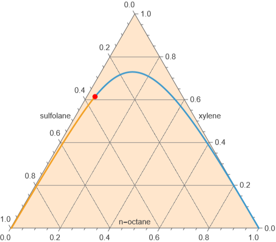
Starting from an initial solution (e.g., for d=0.05) found by FindRoot, the notebook uses NDSolve to continue this solution as a function of the arc-length parameter d(s), producing interpolating functions for x1a(s), x2a(s), x1b(s), x2b(s) and the slopes m1(s), m2(s). This traces the entire two-phase boundary (binodal) in one continuous sweep rather than requiring separate root-finds for each tie line. The plait point (critical point where the two phases merge) is obtained for d(s)=0 and s = - 0.215.
Validation Against Experimental Data
Validation Against Experimental Data
The continuous binodal curve is plotted on a ternary diagram, then overlaid with the 9 experimental tie lines (shown in dashed blue) from Table 2 of Chen et al. (2000) for direct comparison. For each experimental tie line, the notebook computes the arc-length, s, (see mytielinesarclength list) and calculate the corresponding tie line (shown in red). The RMSD between calculated and experimental mole fractions across all tie lines and components is computed; RMSD ≈ 0.0079 confirming good agreement between the continuation-method predictions and the published experimental LLE data.
Method based on common tangent plane and arc-length continuation
In[]:=
ClearAll["Global`*"];
NRTL Model-Chen et al.,Fluid Phase Equilibria 173 (2000)
Parameters at T=298.15 K, Table 3
Parameters at T=298.15 K, Table 3
T=298.15;(*K*)
tau_ij for n-Octane(1)+Xylene(2)+Sulfolane(3), Table 3
τ={{0.0000,-0.3318*10^3,0.2235*10^4},{0.3645*10^3,0.0000,0.4137*10^3},{0.1231*10^4,0.1451*10^3,0.0000}}/T;
Alpha matrix (symmetric)
α={{0,0.2,0.2},{0.2,0,0.2},{0.2,0.2,0}};
In[]:=
α//MatrixForm
Out[]//MatrixForm=
0 | 0.2 | 0.2 |
0.2 | 0 | 0.2 |
0.2 | 0.2 | 0 |
In[]:=
τ//MatrixForm
Out[]//MatrixForm=
0. | -1.11286 | 7.49623 |
1.22254 | 0. | 1.38756 |
4.12879 | 0.486668 | 0. |
In[]:=
G[i_,j_]:=Exp[-α[[i,j]]τ[[i,j]]];
In[]:=
TableForm@Table[G[i,j],{i,1,3},{j,1,3}]
Out[]//TableForm=
1. | 1.24929 | 0.223299 |
0.78309 | 1. | 0.757667 |
0.437903 | 0.907253 | 1. |
Composition vector
xvec[x1_,x2_]:={x1,x2,1-x1-x2};
NRTL activity coefficients
lnGamma[i_,x1_,x2_]:=Module[{x,term1,term2},x=xvec[x1,x2];term1=Sum[x[[j]]τ[[j,i]]G[j,i],{j,1,3}]/Sum[x[[k]]G[k,i],{k,1,3}];term2=Sum[x[[j]]G[i,j]/Sum[x[[k]]G[k,j],{k,1,3}](τ[[i,j]]-Sum[x[[m]]τ[[m,j]]G[m,j],{m,1,3}]/Sum[x[[m]]G[m,j],{m,1,3}]),{j,1,3}];term1+term2];gamma[i_,x1_,x2_]:=Exp[lnGamma[i,x1,x2]];
Dimensionless Gibbs energy of mixing: g/RT
gmix[x1_,x2_]:=Module[{x},x=xvec[x1,x2];Sum[x[[i]]Log[x[[i]]],{i,1,3}]+Sum[x[[i]]lnGamma[i,x1,x2],{i,1,3}]];
Derivatives
dgdx1[x1_,x2_]:=Evaluate[D[gmix[u,v],u]/.{u->x1,v->x2}];dgdx2[x1_,x2_]:=Evaluate[D[gmix[u,v],v]/.{u->x1,v->x2}];
Unknowns
vars={x1a,x2a,x1b,x2b,m1,m2};
Common tangent equations
eq1=dgdx1[x1a,x2a]==m1;eq2=dgdx1[x1b,x2b]==m1;eq3=dgdx2[x1a,x2a]==m2;eq4=dgdx2[x1b,x2b]==m2;eq5=gmix[x1b,x2b]-gmix[x1a,x2a]==m1(x1b-x1a)+m2(x2b-x2a);
Extra constraint - Prevent trivial solution xα=xβ
eq6=(x1b-x1a)^2+(x2b-x2a)^2==d;
First value for d --- very small d=0.001 yield approximately the plait point
d0t=0.05;
Solution
solct=FindRoot[{eq1,eq2,eq3,eq4,eq5,eq6/.d->d0t},{{x1a,0.53},{x2a,0.14},{x1b,0.004},{x2b,0.004},{m1,-1.0},{m2,4}},MaxIterations->10000]//Chop
Out[]=
{x1a0.0716143,x2a0.705186,x1b0.0175396,x2b0.488216,m1-1.58083,m2-0.0306657}
In[]:=
init={x1a[0]==(x1a/.solct),x2a[0]==(x2a/.solct),x1b[0]==(x1b/.solct),x2b[0]==(x2b/.solct),m1[0]==(m1/.solct),m2[0]==(m2/.solct),d[0]==d0t}
Out[]=
{x1a[0]0.0716143,x2a[0]0.705186,x1b[0]0.0175396,x2b[0]0.488216,m1[0]-1.58083,m2[0]-0.0306657,d[0]0.05}
In[]:=
initdev={x1a'[0]==0.0001,x2a'[0]==0.0001,x1b'[0]==0.0001,x2b'[0]==0.0001,m1'[0]==0.01,m2'[0]==0.01,d'[0]==0.001}
Out[]=
{[0]0.0001,[0]0.0001,[0]0.0001,[0]0.0001,[0]0.01,[0]0.01,[0]0.001}
′
x1a
′
x2a
′
x1b
′
x2b
′
m1
′
m2
′
d
In[]:=
SYS={eq1,eq2,eq3,eq4,eq5,eq6}/.x1a->x1a[s]/.x1b->x1b[s]/.x2a->x2a[s]/.x2b->x2b[s]/.m1->m1[s]/.m2->m2[s]/.d->d[s];
In[]:=
auxeq=x1a'[s]^2+x1b'[s]^2+x2a'[s]^2+x2b'[s]^2+m1'[s]^2+m2'[s]^2+d'[s]^2==1;
In[]:=
SYSFinal=Join[SYS,{auxeq},init,initdev];
SOL=Quiet@NDSolve[SYSFinal,{x1a,x2a,x1b,x2b,m1,m2,d},{s,-10,10},AccuracyGoal->10];
In[]:=
DATA1=Table[{x1a[s],x2a[s],1-x1a[s]-x2a[s]}/.SOL,{s,-0.215,10,0.001}];DATA2=Table[{x1b[s],x2b[s],1-x1b[s]-x2b[s]}/.SOL,{s,-0.215,10,0.001}];
In[]:=
Pt={{2,1},{0,Sqrt[3.]}}/2;
Type I liquid-liquid equilibrium (LLE) diagram - Plait point indicated in red
In[]:=
FindRoot[(d[s]/.SOL)==0.00001,{s,-0.2}]
Out[]=
{s-0.214023}
In[]:=
p0=Show[TernaryListPlot[{Flatten[DATA1,1],Flatten[DATA2,1]},Joined->True,PlotStyle->Thick,GridLines->Automatic,FrameLabel->{"n-octane","xylene","sulfolane"},PlotRange->All,Method->{"Backdrop"->LightOrange}],Graphics[{Red,PointSize[0.02],Point[Pt.{x1a[s],x2a[s]}/.SOL/.s->-0.2140]}]]
Out[]=
Octane-rich phase {x1,x2,x3}, Sulfolane-rich phase {x1,x2,x3}
Octane-rich phase {x1,x2}, Sulfolane-rich phase {x1,x2}
Octane-rich phase {x1,x2}, Sulfolane-rich phase {x1,x2}
tieLines={{{0.831,0.165},{0.007,0.048}},{{0.752,0.242},{0.007,0.063}},{{0.677,0.318},{0.008,0.087}},{{0.609,0.381},{0.009,0.106}},{{0.547,0.436},{0.009,0.125}},{{0.486,0.494},{0.010,0.145}},{{0.429,0.541},{0.013,0.199}},{{0.312,0.640},{0.014,0.231}},{{0.262,0.672},{0.015,0.267}}};octaneRich=Table[tieLines[[i]][[1]],{i,1,9}];sulfolaneRich=Table[tieLines[[i]][[2]],{i,1,9}];
Add x3 column (water/acetate,by difference) and full triples
octaneRichFull=Map[Append[#,1-Total[#]]&,octaneRich];sulfolaneRichFull=Map[Append[#,1-Total[#]]&,sulfolaneRich];
Display as tables with headers
TableForm[octaneRichFull,TableHeadings->{None,{"x1 (n-octane)","x2 (xylene)","x3 (sulfolane)"}}]TableForm[sulfolaneRichFull,TableHeadings->{None,{"x1 (n-octane)","x2 (xylene)","x3 (sulfolane)"}}]
Out[]//TableForm=
x1 (n-octane) | x2 (xylene) | x3 (sulfolane) |
0.831 | 0.165 | 0.004 |
0.752 | 0.242 | 0.006 |
0.677 | 0.318 | 0.005 |
0.609 | 0.381 | 0.01 |
0.547 | 0.436 | 0.017 |
0.486 | 0.494 | 0.02 |
0.429 | 0.541 | 0.03 |
0.312 | 0.64 | 0.048 |
0.262 | 0.672 | 0.066 |
Out[]//TableForm=
x1 (n-octane) | x2 (xylene) | x3 (sulfolane) |
0.007 | 0.048 | 0.945 |
0.007 | 0.063 | 0.93 |
0.008 | 0.087 | 0.905 |
0.009 | 0.106 | 0.885 |
0.009 | 0.125 | 0.866 |
0.01 | 0.145 | 0.845 |
0.013 | 0.199 | 0.788 |
0.014 | 0.231 | 0.755 |
0.015 | 0.267 | 0.718 |
Combine into tie-line pairs:{phaseI,phaseII}
Show all nine experimental tie lines
Let us compute the RMSD
Reference
Reference
[1] J. Chen, L.-P. Duan, J.-G. Mi, W.-Y. Fei, Z.-C. Li, “Liquid–liquid equilibria of multi-component systems including n-hexane, n-octane, benzene, toluene, xylene and sulfolane at 298.15 K and atmospheric pressure,” Fluid Phase Equilibria, Vol. 173, 2000, pp. 109–119. DOI/PII: S0378-3812(00)00398-8
CITE THIS NOTEBOOK
CITE THIS NOTEBOOK
Liquid–liquid equilibrium calculation for the n-octane + xylene + sulfolane system
by Housam Binous
Wolfram Community, STAFF PICKS, June 28, 2026
https://community.wolfram.com/groups/-/m/t/3740609
by Housam Binous
Wolfram Community, STAFF PICKS, June 28, 2026
https://community.wolfram.com/groups/-/m/t/3740609