Ellipse errors
Ellipse errors
In[]:=
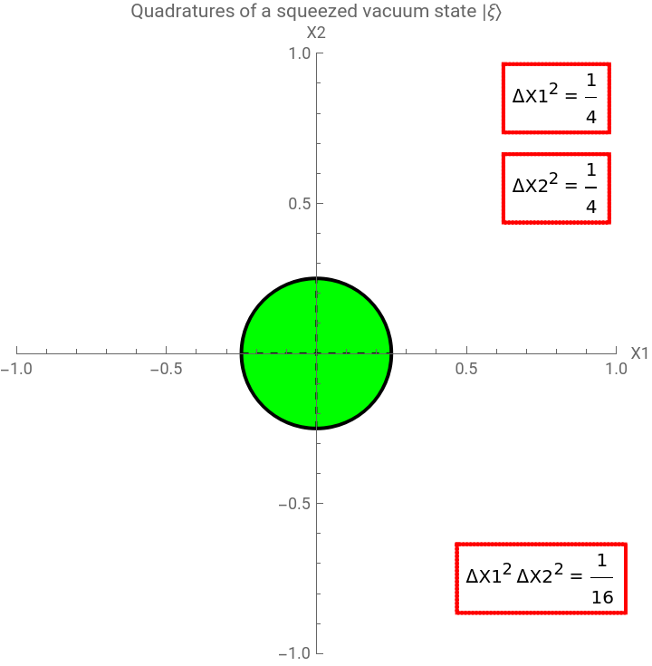
ManipulateModule{dx=1/4Exp[-2r],dy=1/4Exp[2r]},GraphicsEdgeForm[Thick],Green,Rotate[Disk[{0,0},{dx,dy}],θ1/2],Black,Dashed,Line[Outer[Times,{-dx,dx},{Cos[θ1/2],Sin[θ1/2]}]],Line[Outer[Times,{-dy,dy},{-Sin[θ1/2],Cos[θ1/2]}]],TextFramed==14(+-2Sinh[r]Cosh[r]Cos[θ1]),FrameStyle->Directive[Red,Thick,Dashing[0,0,0]],{0.8,0.85},TextFramed==14(++2Sinh[r]Cosh[r]Cos[θ1]),FrameStyle->Directive[Red,Thick,Dashing[0,0,0]],{0.8,0.55},TextFramed==116(-),FrameStyle->Directive[Red,Thick,Dashing[0,0,0]],{0.75,-0.75},Axes->True,ImageSize->Medium,AxesLabel->{"X1","X2"},PlotRange->{{-1,1},{-1,1}},PlotLabel->"Quadratures of a squeezed vacuum state |ξ〉",{{r,0,"Modulus r"},0,1},{{θ1,0,"Argument θ"},0,2π},SaveDefinitions->True
2
(ΔX1)
2
Cosh[r]
2
Sinh[r]
2
(ΔX2)
2
Cosh[r]
2
Sinh[r]
2
(ΔX1)
2
(ΔX2)
2
(+)
2
Cosh[r]
2
Sinh[r]
2
(2Sinh[r]Cosh[r]Cos[θ1])
Out[]=


Poll Question #2: Single photon interference (non balanced BS)
Poll Question #2: Single photon interference (non balanced BS)
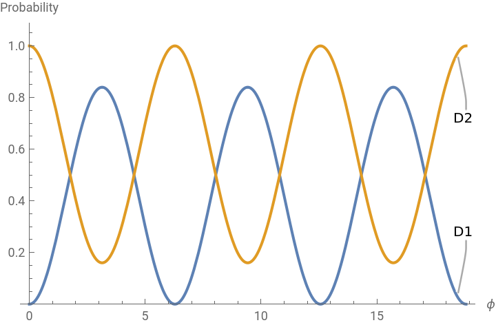
Actually this one was not worded properly, so i apologize if it was confusing. If BOTH beam splitter are changed to non balanced, the probabilities will never reach zero BUT only at one of the output ports. The case i was referring to is when only one of the beam-splitter is changed to non balanced.
Both non balanced
Both non balanced
In[]:=
SetFockSpaceSize[3];
In[]:=
a5=a;a6=QuantumOperator[a,{2}];
We now use a dielectric beam splitter (non balanced):
In[]:=
nonbalancedBS=GeneralBSArcCos[
3/10
],0,0,0;Compute the operator of the arrangement:
In[]:=
MZ=nonbalancedBS@QuantumOperator["P"[ϕ]]@nonbalancedBS;
Relating the final and initial operators (Heisenberg-like evolution):
In[]:=
{a1,a2}=Inverse@MZ["Matrix"].{a5,a6};
In[]:=
probs=(a1["Dagger"]@FockState[{0,0}])["Probability"]
Out[]=
01+,10+
2Im[ϕ]
2
Abs-+
21
10
1
10
21
-Conjugate[ϕ]
2Im[ϕ]
2
Abs+
3
10
7
10
-Conjugate[ϕ]
2Im[ϕ]
2
Abs-+
21
10
1
10
21
-Conjugate[ϕ]
2Im[ϕ]
2
Abs+
3
10
7
10
-Conjugate[ϕ]
2Im[ϕ]
2
Abs+
3
10
7
10
-Conjugate[ϕ]
2Im[ϕ]
2
Abs-+
21
10
1
10
21
-Conjugate[ϕ]
In[]:=
simplifiedProbs=FullSimplify[probs//Values,Element[ϕ,Reals]]//ComplexExpand//TrigReduce
Out[]=
-(-1+Cos[ϕ]),(29+21Cos[ϕ])
21
50
1
50
In[]:=
Plot[Evaluate@MapThread[Callout[#1,#2,Right]&,{simplifiedProbs,{"D1","D2"}}],{ϕ,0,6Pi},AxesLabel->{"ϕ","Probability"},PlotLegends->{"Output 5","Output 6"},PlotRange->{0,1}]
Out[]=


In[]:=
Total[simplifiedProbs]//Simplify
Out[]=
1
Only one non balanced
Only one non balanced
In[]:=
balancedBS=GeneralBS[π/4,0,0,0];MZ=nonbalancedBS@QuantumOperator["P"[ϕ]]@balancedBS;{a1,a2}=Inverse@MZ["Matrix"].{a5,a6};
In[]:=
probs=(a1["Dagger"]@FockState[{0,0}])["Probability"]
Out[]=
01+,10+
2Im[ϕ]
2
Abs-+
7
5
2
1
2
3
5
-Conjugate[ϕ]
2Im[ϕ]
2
Abs-+
7
5
2
1
2
3
5
-Conjugate[ϕ]
2Im[ϕ]
2
Abs+
3
5
2
1
2
7
5
-Conjugate[ϕ]
2Im[ϕ]
2
Abs+
3
5
2
1
2
7
5
-Conjugate[ϕ]
2Im[ϕ]
2
Abs-+
7
5
2
1
2
3
5
-Conjugate[ϕ]
2Im[ϕ]
2
Abs+
3
5
2
1
2
7
5
-Conjugate[ϕ]
In[]:=
simplifiedProbs=FullSimplify[probs//Values,Element[ϕ,Reals]]//ComplexExpand//TrigReduce
Out[]=
5-5+
1
10
21
Cos[ϕ],1
10
21
Cos[ϕ]In[]:=
Plot[Evaluate@MapThread[Callout[#1,#2,Right]&,{simplifiedProbs,{"D1","D2"}}],{ϕ,0,6Pi},AxesLabel->{"ϕ","Probability"},PlotLegends->{"Output 5","Output 6"},PlotRange->{0,1}]
Out[]=
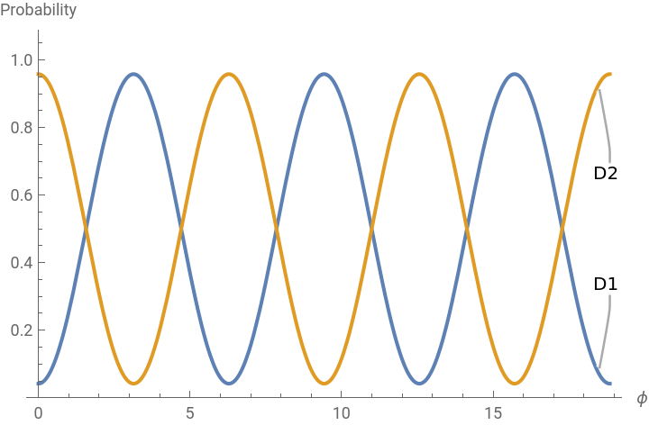
For this case the minimum is (5 ) that is not zero, that will change depending on how asymmetric is the non balanced beam-splitter.
1
10
-
21
In[]:=
Minimize[#,ϕ][[1]]&/@simplifiedProbs
Comments and Questions
Comments and Questions
Question:
Question:
How are quasiprobability functions calculated? Using the fast Fourier transform or with the series given as an exercise in Peter Knight’s book?”
Answer:
Answer:
I answered during the class, but i wanted to say it more explicitly. The Wigner function is calculated using Clenshaw recurrence to evaluate Laguerre polynomials in a faster way. The Husimi Q function does not use any particular algorithm, it is just based on the definition shown on the class but with some numerical improvements regarding speed.