ORIGINAL ARTICLE: Khodabaccus, N., Saib, A.A.E.F. volatilityforecastingpackage: A Financial Volatility Package in Mathematica. Comput Econ (2023). DOI: https://doi.org/10.1007/s10614-023-10406-2
Abstract: We introduce the volatilityforecastingpackage for financial volatility modelling and forecast visualisation using state-of-the art algorithms. This package allows recourse to algorithms through a user friendly interface that provides easy access to models for high and low frequency data, while accessibly generating forecasts, estimating errors and plots. The package also allows analysis of user data and based on the results, a set of models appropriate for the data type may eventually be used in the modelling.
■
Introduction
Introduction
Volatility in the financial market refers to the fluctuation of returns for assets and usually implies that a high level of risk is present (Chen et al. 2023). As a result, soaring levels of volatility in the financial markets are capable of having a negative impact on risk averse investors. Hence, the fair modelling of volatility provides a critical input in many empirical fields including risk management, portfolio selection and derivative pricing. Also, due to the financial linkages of the global economy and foundation of various trade unions, the correlation between different economies lead to an eroding portfolio diversification, thus increasing the threat of volatility transmission, also known as the volatility spillover effect (Enderwick & Buckley 2020, Son et al. 2023).
Since volatility cannot be directly observed, it has to be estimated using appropriate mathematical models. Several methods for volatility forecasting have been proposed in the literature but that usually does not corroborate with their easy access to end-users, like practitioners. Software packages or functions have in the sequel been proposed and for instance, in Mathematica, volatility can be forecasted using the inbuilt GARCHProcess function. We extend the time series functions provided under the Mathematica framework and propose a dedicated package which caters for different types of data, while also providing access to machine learning approaches which are suitable for large datasets . Incomplete or scarce data sets with no prior assumption on probability distributions are catered by some grey models.
Since volatility cannot be directly observed, it has to be estimated using appropriate mathematical models. Several methods for volatility forecasting have been proposed in the literature but that usually does not corroborate with their easy access to end-users, like practitioners. Software packages or functions have in the sequel been proposed and for instance, in Mathematica, volatility can be forecasted using the inbuilt GARCHProcess function. We extend the time series functions provided under the Mathematica framework and propose a dedicated package which caters for different types of data, while also providing access to machine learning approaches which are suitable for large datasets . Incomplete or scarce data sets with no prior assumption on probability distributions are catered by some grey models.
□
Package Installation & Loading
Package Installation & Loading
The package (attached below) must be installed either in the User Base Directory or the Base Directory and can be loaded using either one of the following commands:
<<thevolatilityforecastingpackage`, Get[“thevolatilityforecastingpackage`”], or Needs[“thevolatilityforecastingpackage`”].
<<thevolatilityforecastingpackage`, Get[“thevolatilityforecastingpackage`”], or Needs[“thevolatilityforecastingpackage`”].
In[]:=
<<thevolatilityforecastingpackage`
Welcome to the volatility forecasting package
The volatility forecasting package has been created using Mathematica version 12.2. The inbuilt functions may be viewed by evaluating ?volatilityforecastingpackage`*.
In[]:=
?volatilityforecastingpackage`*

Usage information is available on clicking any of the respective inbuilt function
□
Loading the dataset to check the volatility
Loading the dataset to check the volatility
The VolatilityForecastingPackage allows users to either load their own dataset (the package directly supports data stored in comma separated variable (.csv) format or allows use of financial data from the Wolfram database.
1. To check the volatility of their dataset, the user follows:
1. To check the volatility of their dataset, the user follows:
Out[]=
Test Case 1
Suppose a user want to load and calculate the volatility of Bitcoin from August, 12, 2022 - August, 12, 2023 using inbuilt functions in the package.
In[]:=
CheckVolatility[input1]
Out[]=
The dataset loaded may be classified as high frequency and high volatility data and the models appropriate for your data type are: ARIMA, ForecastWithMachineLearning, garch, garchT, GeometricBrownianMotion, GjrGarch, GjrGarchT, RidgeRegression,RNN
2. To check the volatility of financial data from the Wolfram database, a user follows:
Out[]=
Test Case 2
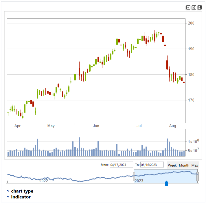
The volatility of APPL stocks from August,12,2022 - August,12,2023 is presented below:
In[]:=
CheckVolatility[input1]
The dataset loaded may be classified as low frequency and low volatility data and the models appropriate for your data type are: FAGM11, FANGBM, GM11, GM1N, NGBM, OpNGBM, PSOGM11
□
Calculating the confidence interval
Calculating the confidence interval
The VolatilityForecastingPackage allows a user to visualise forecasts alongside the confidence interval plots. Since the package has models suitable for both high and low frequency data, the confidence intervals are calculated according to:
CI=
|
where CI is the confidence interval, FV is forecasted value, α is the chosen confidence level, s is the standard deviation and n is the number of elements in the dataset.
◼
Some Inbuilt Models In The Package
Some Inbuilt Models In The Package
The models in the VolatilityForecastingPackage are divided into 2 categories namely, models suitable for high frequency data and models suitable for low frequency data.
□
Models for high frequency data
Models for high frequency data
The following are inbuilt functions for data classified as having high frequency: RidgeRegression, MLalgo, RNN, GBM, Garch, GarchT, GjrGarch and GjrGarchT, LSTM and BiLSTM.
As an example, to use the Ridge regression, run
Out[]=
Data should be in the form {{x1, v1}, {x2, v2}, . . . , {xi, vi}}, where xi and vi are the input 1 and 2 respectively, for instance, they can be the first 2 columns in the spreadsheet.
The RidgeRegression[input1, input2] function gives the user the forecasted values and also outputs the plot.
The RidgeRegression[input1, input2] function gives the user the forecasted values and also outputs the plot.
Test Case 3
We use the RidgeRegression[input1, input2] function to identify any relationship between the opening and closing price of Brent crude oil from August 17, 2022 - September 17, 2023.
In[]:=
Dataselection[bcc]
Out[]=
NotebookObject

In[]:=
RidgeRegression[input1,input2]
Out[]=
We also give as example, the GBM model which may be called using:
Out[]=
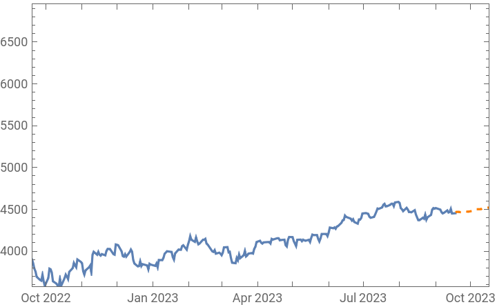
To employ the neural network model for forecasting Standard and Poor’s 500 financial data from September, 18, 2022 - September, 18, 2023 , we evaluate:
GBM[input1]
Out[]=
If conventional time series are required, we may resort for instance to the ARIMA model which may be called using:
Test case 4
As an example, to employ the ARIMA model for forecasting historical AUD/USD foreign exchange data from June , 28, 2016 - July, 11, 2023, we evaluate:
Machine learning techniques
Machine learning techniques
Some machine learning techniques are as well inbuilt in the package. In particular, the MLalgo[input] function allows users to forecast volatility using machine learning techniques such as Gaussian process, linear regression, k - nearest neighbours, artificial neural networks (ANN), decision trees, gradient boosted trees and random forest. To use any of the aforementioned models, the user is expected to follow:
Test case 5
As an example, to employ the neural network model for forecasting historical AUD/USD foreign exchange data from 28th June 2016 - 11th July 2023 , evaluate:
Deep learning approaches
Deep learning approaches
Some deep learning approaches such as the recurrent neural network (RNN), LSTM and BiLSTM are as well included in the package. To use the BiLSTM model for high volatility forecasting, the user is expected to follow:
Test Case 6
As an example, the BiLSTM is employed to forecast historical gold futures data from June 15, 2013 - Jul, 13, 2023
GARCH type models
GARCH type models
Two GARCH type models are included in the VolatilityForecastingPackage, namely GARCH (1, 1) and the GJR GARCH with both normal and student's t - distributions. To forecast volatility using the GARCH (1, 1), the user follows :
Test case 7
As an example, to employ the Garch model for forecasting the volatility of the historical AUD/USD foreign exchange data from June 28, 2016 - July 11, 2023 , we evaluate :
The same steps should be followed for forecasting volatility with the GARCH (1, 1) with student’s - t distribution and the GJR GARCH models with both normal and student’s- t distributions.
◻
Models for low frequency data
Models for low frequency data
The volatility forecasting package also accommodates forecasts for small/scarce/incomplete historical datasets. The models implemented are:
grey model (GM11), multi variable grey model (GM1N), non-linear grey Bernoulli model (NGBM), Optimized GM(1, 1) model with both particle swarm optimization and firefly algorithm (PSOGM and FAGM11), optimized NGBM with firefly algorithm (FANGBM).
grey model (GM11), multi variable grey model (GM1N), non-linear grey Bernoulli model (NGBM), Optimized GM(1, 1) model with both particle swarm optimization and firefly algorithm (PSOGM and FAGM11), optimized NGBM with firefly algorithm (FANGBM).
Univariate grey models
Univariate grey models
To evaluate the GM (1, 1),
Test case 8
As an example, to employ the grey model for forecasting the energy demand consumption in Mauritius for the period 2010 - 2019, we evaluate:
As another test case, the user may employ the optimised NGBM (1, 1). The nonlinear grey Bernoulli model, NGBM(1, 1), is the isomorphism of the traditional GM(1, 1) and an ordinary differential equation.
To use the model, the user executes:
To use the model, the user executes:
Test case 9
Optimisation of some volatility forecasting models using metaheuristics algorithms
Optimisation of some volatility forecasting models using metaheuristics algorithms
Since metaheuristics algorithms are powerful tools for modelling and optimisation of parameters, the PSO and FA were implemented to enhance the prediction results of the grey models.
To call the FAGM11 model, the user needs to:
◼
Grey Models And Markov Chains
Grey Models And Markov Chains
The Markov Chain Grey Model (MCGM)
The Markov Chain Grey Model (MCGM)
The grey prediction models can be merged with the concept of Markov chains to enhance their performance, with the latter usually used to predict time series data (Zhan - li & Jinhua 2011). To call the MCGM model, the user needs to:
Test case 10
To use the MCGM model, evaluate:
Markov chain non-linear grey Bernoulli model (MCNGBM)
Markov chain non-linear grey Bernoulli model (MCNGBM)
The Markov chain non - linear grey Bernoulli further improves the predictive accuracy of the optimised NGBM model. To call the MCNGBM model, the user needs to:
Test case 11
To use the MCNGBM model, evaluate :
◻
Fourier series, Markov chains and firefly optimised grey models.
Fourier series, Markov chains and firefly optimised grey models.
The Fourier-Markov optimised grey model (FOGM).
The Fourier-Markov optimised grey model (FOGM).
Fourier can be employed to improve the forecasting performance of random and uncontrolled data since they can be used to analyse oscillating sequences (Wang et al. 2021, Khodabaccus & Saib, 2023).
To call the FOGM model, the user needs to :
To call the FOGM model, the user needs to :
Test case 12
■
Conclusion
Conclusion
The VolatilityForecastingPackage allows users and practitioners alike to have an easy recourse to some state-of-the-art algorithms through a user friendly interface for modelling financial volatility. The package allows users to have access to models suitable for both high and low frequency data. A benchmark check of the volatility and frequency of a dataset is implemented and shown that based on the results, appropriate models are then recommended.
References
References
1. ChenWJ, Yao JJ, Shao YH.Volatility forecasting using deep neural network with time - series feature embedding.Economic Research - Ekonomska Istraživanja .2023; 36 (1) : 1377–1401.
2. Enderwick P, Buckley PJ. Rising regionalization : will the post - COVID - 19 world see a retreat from globalization?. Transnational Corporations Journal. 2020; 27 (2).
3. Son B, Lee Y, Park S, Lee J. Forecasting global stock market volatility : The impact of volatility spillover index in spatial - temporal graph - based model. Journal of Forecasting. 2023;
4. Zhan - li, M. and Jin - hua, S. (2011) ' Application of grey - Markov model in forecasting fire accidents', Procedia Engineering, Vol. 11, pp .314–318 .
5. Wang, Z. and Wang, H. (2021) ' Improving load forecast in energy markets during COVID - 19', in Proceedings of the 8th ACM International Conference on Systems for Energy - Efficient Buildings, Cities, and Transportation, ACM.
6. Khodabaccus N, Saib A. Energy Demand Forecasting Using A Novel Optimised Fourier Grey Markov Based Approach. International Journal of Operational Research. 2023; 1(in press).
CITE THIS NOTEBOOK
CITE THIS NOTEBOOK
volatilityforecastingpackage: A Financial Volatility Package in Mathematica
by Noorshanaaz Khodabaccus and Aslam Saib
Wolfram Community, STAFF PICKS, September 27, 2023
https://community.wolfram.com/groups/-/m/t/3022818
by Noorshanaaz Khodabaccus and Aslam Saib
Wolfram Community, STAFF PICKS, September 27, 2023
https://community.wolfram.com/groups/-/m/t/3022818