Wolfram Cloud Document

We propose to find all azeotropes for a pentanary mixture composed of Ethanol, Benzene, Chloroform, Acetone and Methanol at 1 atm using the Wilson model.This problem was first treated by Fidkowski, Malone and Doherty (Ref. 1) and their results are reproduced below:

Finally, this problem was also investigated by the late Prof. Floudas and co-workers using GAMS: see Chapter 14 at : http://titan.princeton.edu/TestProblems/

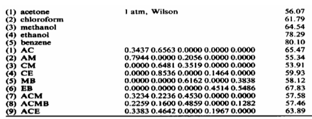
This system has 9 azeotropes (6 binary azeotropes + 2 ternary azeotropes + 1 quaternary azeotrope).

We benchmark our results, summarized in the Table below, against data generated by Aspen-Properties as well as a Matlab bifurcation code written by several people at the CHE department of MIT including the late Prof. Swan.

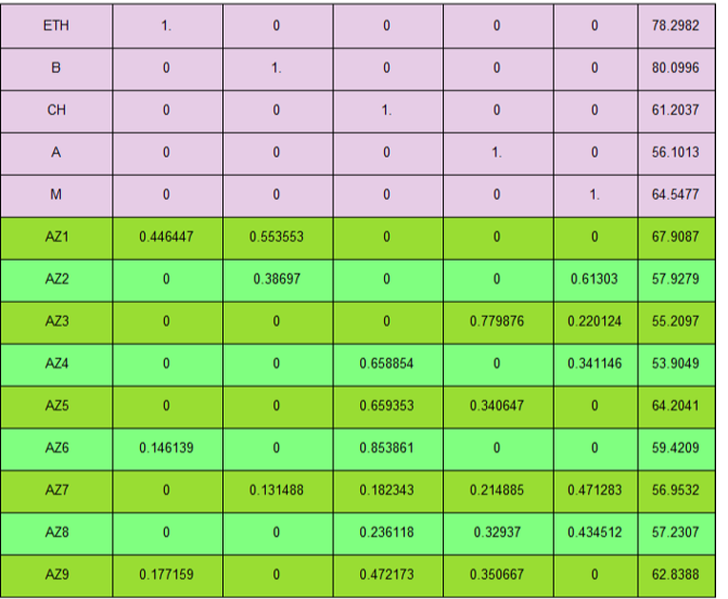
Ethanol = component 1
Benzene = component 2
Chloroform = component 3
Acetone = component 4
Methanol = component 5

In[]:=

(*vaporpressureofallcomponentsusingAnotineEquationTisinKelvinandpessureisinmmHg*)p1[T_]:=10^(8.11220-1592.864/(226.184+(T-273.15)));(*ethanol*)p2[T_]:=10^(6.87987-1196.760/(219.161+T-273.15));(*benzene*)p3[T_]:=10^(6.95465-1170.966/(226.232+T-273.15));(*chloroform*)p4[T_]:=10^(7.11714-1210.595/(-43.486+T));(*acetone*)p5[T_]:=10^(8.08097-1582.271/(-33.424+T));(*methanol*)P=760;(*totalpressureinmmHg*)(*Temperature-dependentparametersofWilsonmodelarereproducedfromAspen-Properties*)A={{0,1.0936,0.,0.7465,-4.0246},{0.0106,0,-2.4936,0.0849,5.0726},{0.,1.2772,0,-0.7191,0.},{0.8542,-0.4336,-0.7683,0,0.},{1.5166,-9.6962,0.,0.,0}};B={{0,-958.013,-591.401,-346.039,991.718},{-232.531,0,589.487,-237.196,-2040.48},{36.5424,-188.941,0,435.144,-32.5972},{-405.215,184.624,262.179,0,-115.663},{-288.173,2571.88,-652.896,-108.526,0}};wilson[x_,T_]:=Module[{Lambdas,gammas,i,j},For[i=1,i≤5,i++,For[j=1,j≤5,j++,Lambdas[i,j]=Exp[A[[i,j]]+B[[i,j]]/(T)]]];For[i=1,i≤5,i++,gammas[i]=1-Log[Sum[Lambdas[i,k]x[[k]],{k,1,5}]];For[j=1,j≤5,j++,gammas[i]=gammas[i]-Lambdas[j,i]x[[j]]/Sum[Lambdas[j,k]x[[k]],{k,1,5}]]];Table[Exp[gammas[i]],{i,1,5}]]myPsats[T_]:={p1[T],p2[T],p3[T],p4[T],p5[T]};mysyshom[x_,T_,l_]:=Module[{gammas,psat},gammas=wilson[x,T];psat=myPsats[T];{x[[1]]-((1-l)+lgammas[[1]])psat[[1]]x[[1]]/P0,x[[2]]-((1-l)+lgammas[[2]])psat[[2]]x[[2]]/P0,x[[3]]-((1-l)+lgammas[[3]])psat[[3]]x[[3]]/P0,x[[4]]-((1-l)+lgammas[[4]])psat[[4]]x[[4]]/P0,x[[5]]-((1-l)+lgammas[[5]])psat[[5]]x[[5]]/P0,x[[1]]+x[[2]]+x[[3]]+x[[4]]+x[[5]]-10}]

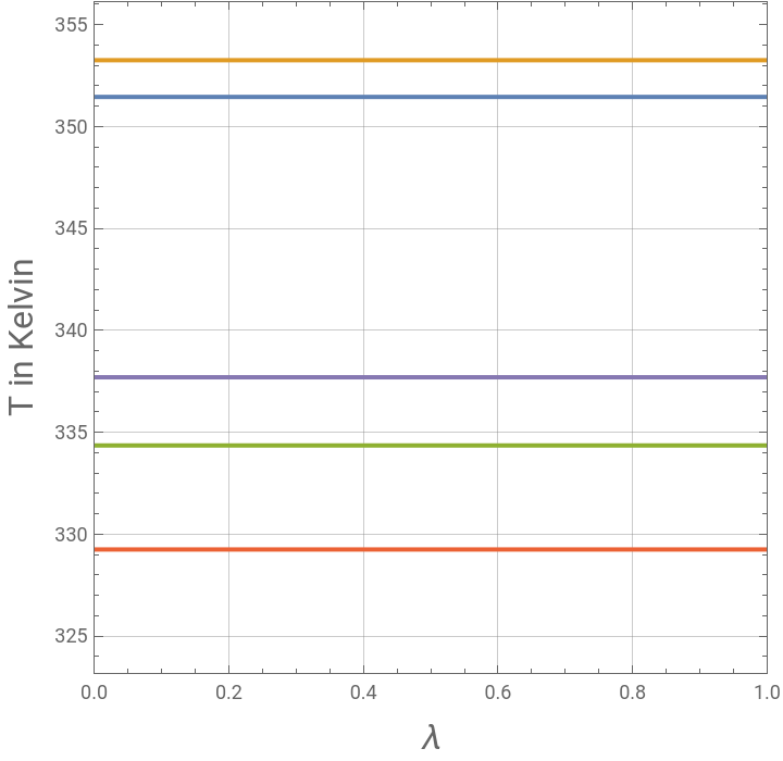
Pure components' boiling point versus λ

In[]:=

l=Table[i,{i,0,1,0.01}];data=.;guess={1,10^-12,10^-12,10^-12,10^-12,360};data[1]=Table[{l[[i]],T/.Quiet@FindRoot[mysyshom[{x1,x2,x3,x4,x5},T,l[[i]]],{x1,guess[[1]]},{x2,guess[[2]]},{x3,guess[[3]]},{x4,guess[[4]]},{x5,guess[[5]]},{T,guess[[6]]}]},{i,1,101}];guess={10^-12,1,10^-12,10^-12,10^-12,360};data[2]=Table[{l[[i]],T/.Quiet@FindRoot[mysyshom[{x1,x2,x3,x4,x5},T,l[[i]]],{x1,guess[[1]]},{x2,guess[[2]]},{x3,guess[[3]]},{x4,guess[[4]]},{x5,guess[[5]]},{T,guess[[6]]}]},{i,1,101}];guess={10^-12,10^-12,1,10^-12,10^-12,360};data[3]=Table[{l[[i]],T/.Quiet@FindRoot[mysyshom[{x1,x2,x3,x4,x5},T,l[[i]]],{x1,guess[[1]]},{x2,guess[[2]]},{x3,guess[[3]]},{x4,guess[[4]]},{x5,guess[[5]]},{T,guess[[6]]}]},{i,1,101}];guess={10^-12,10^-12,10^-12,1,10^-12,360};data[4]=Table[{l[[i]],T/.Quiet@FindRoot[mysyshom[{x1,x2,x3,x4,x5},T,l[[i]]],{x1,guess[[1]]},{x2,guess[[2]]},{x3,guess[[3]]},{x4,guess[[4]]},{x5,guess[[5]]},{T,guess[[6]]}]},{i,1,101}];guess={10^-12,10^-12,10^-12,10^-12,1,360};data[5]=Table[{l[[i]],T/.Quiet@FindRoot[mysyshom[{x1,x2,x3,x4,x5},T,l[[i]]],{x1,guess[[1]]},{x2,guess[[2]]},{x3,guess[[3]]},{x4,guess[[4]]},{x5,guess[[5]]},{T,guess[[6]]}]},{i,1,101}];

In[]:=

plt=ListPlot[{data[1],data[2],data[3],data[4],data[5]},GridLinesAutomatic,FrameTrue,AspectRatio1,Joined->True,PlotRange{{0,1},{50+273.15,83+273.15}},FrameLabel{Style["λ",16],Style["T in Kelvin",16]}]

Out[]=

Approach based on changing each time the initial guess in order to find the corresponding azeotropes .
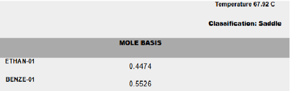
As shown below, this approach compares favorably with Aspen - Properties output .

Aspen output for the pentanry system

In[]:=

guess={0.4,0.6,0.0,0.0,0.0,320};FindRoot[mysyshom[{x1,x2,x3,x4,x5},T,1],{x1,guess[[1]]},{x2,guess[[2]]},{x3,guess[[3]]},{x4,guess[[4]]},{x5,guess[[5]]},{T,guess[[6]]}]

Out[]=

{x10.446447,x20.553553,x32.69049×

-40

,x4-6.2554×

-42

,x56.09845×

-41

,T341.059}

Aspen output for the pentanry system

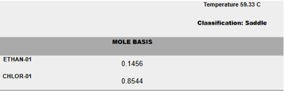
In[]:=

guess={0.4,0.0,0.6,0.0,0.0,320};FindRoot[mysyshom[{x1,x2,x3,x4,x5},T,1],{x1,guess[[1]]},{x2,guess[[2]]},{x3,guess[[3]]},{x4,guess[[4]]},{x5,guess[[5]]},{T,guess[[6]]}]

Out[]=

{x10.146139,x2-8.84871×

-27

,x30.853861,x40.,x57.07538×

-33

,T332.571}

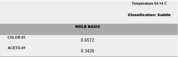
Aspen output for the pentanry system

Bifurcation Approach inspired from Matlab code by CHE Depart. of MIT

1st branch

2nd branch

3rd branch

4th branch

5th branch

6th branch

7th branch

8th branch

9th branch

Comparison with output from MIT code (created by several peoples at the CHE Dept. of MIT including the late Prof. Swan)

MATLAB OUTPUT (Code created by several peoples at the CHE Dept . of MIT including the late Prof . Swan)

All seven azeotropes

References

[1] Z.T. Fidkowski, M.F. Malone, M.F. Doherty, Computing azeotropes in multicomponent mixtures, Computers & Chemical Engineering, Volume 17, Issue 12, 1993, Pages 1141-1155, https://doi.org/10.1016/0098-1354(93)80095-5

CITE THIS NOTEBOOK

All azeotropes of a pentanary system by bifurcation
by Housam Binous and Ahmed Bellagi
Wolfram Community, STAFF PICKS, July 7, 2025
https://community.wolfram.com/groups/-/m/t/3492320